Week 4 - Genetic Algorithm

Aim

To write a code to find the global maxima value for the given stalagmite function using Genetic algorithm (ga) in matlab.

About Genetic Algorithm

• Genetic algorithm is generally reflects the process of natural selection . it was proposed by Charles Darwin
• Basically GA is a search based optimization method in a set of inputs.
• It follows the principle of Natural selection in terms of biological .
• GA generally picks two random individuals in a search space to produce a offspring.
• So the random individuals, ie the parents of the offspring selection is purely based on their fitness value which gives high percentage solutions to the problems
• So highest fitness value offspring is produced
• It has a workflow for this process. Initialization is the very first process where it selects the random individuals and evaluate the fitness value in evaluation process
• The process Optimization with the inputs runs in the below given loop
• Genetic algorithm is used for high quality solutions by relying on following operators

1. Mutations
2. crossover
3. selection

• when the offspring comes out with better fitness value or highest fitness value the loop stops and give it as Best solution

Formulae used

• `〖F1=[sin⁡(5.1πx+0.5) ]〗^6`
• `〖F2=[sin⁡(5.1πy+0.5) ]〗^6`
• `F3=exp⁡[((-4 ln⁡〖(2)×((x-0.0667)^2 )〗 ))/0.64]`
• `F4=exp⁡[((-4 ln⁡〖(2)×((y-0.0667)^2 )〗 ))/0.64]`
• `f=-(f1*f2*f3*f4)`

PROCEDURE

• initially search space is provided for the inputs with 150 values using linspace command
• no of iteration is provided for the function
• The function is coded for given stalagmite problem
• This stalagmite function is a test function to test the ga optimizing technique. That is to find the global maxima
• In our stalagmite function for f value we have to use a negative sign to invert the surface plot
• This because we know that GA is only used to find the global minima value
• We use for loop to get value for function
• And the function runs with the input vectors and gives value of F
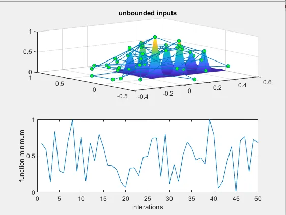
• At first we have to test the function in ga with unbounded condition
• We run the for loop with ga command using the two variables as input
• We get xopt and yopt which can plotted in upcoming code
• We use tic and toc command to get individual study time
• We plotted the optimize values inscribed with in the surface plot of the stalagmite function
• We get randomly optimized points all over the surface but it did not specifiy the global maxima
• we have used negative signs to upright the surface stalagmite for better view of results
• in casing of plotting we use subplot command to get the 2 graphs at same window
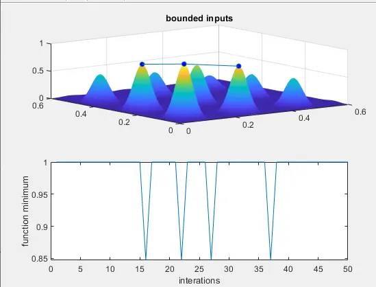
• Next case is providing boundary conditions
• In this study we provide the boundary limit . This boundary limits helps the ga command to optimize under a specified boundary limits
• Here we can get more optimized results but still it doesn’t shows the exact global maxima
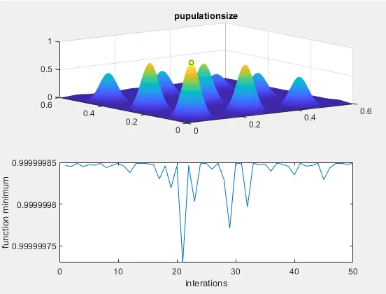
• So in the next study we use population size to take more iteration to figure it out the global maxima
• And finally ga comes to stopping criteria/best solution and the loop stops running
• Time taken for study 1=6.98sec
• Time taken for study2=7.4sec
• Time taken for study3=38.9sec
• Tic toc command used to find this

SYNTAX EXPLAINED

• in the first case we use ga command and we call the function with two variables
• in second case we use ga command ,we call our function with two variables and we use [] square set brackets .
• these set brackets are used when no non linear equilibrium (aeq ,beq)are gives and at last we use boundary condition
• similarly in last case we add population size for better accuracy in the solution

Output

case 1 unbounded condition

case2 bounded condition

case 3 bounded condition with population size

Conclusion

Thus we have found the global maxima of the stalagmite function using ga command

clear all
close all
clc


%search space 


x=linspace(0,0.6,150);
y=linspace(0,0.6,150);
num=50;
[xx yy]=meshgrid(x,y)
for i=1:length(xx);
    for j=1:length(yy);
        ip_vector(1)= xx(i,j);
        ip_vector(2)= yy(i,j);
        
        f(i,j)=stalagmite(ip_vector);
        
    end
end

% study 1 unbounded condition,where no boundry condition is provided 

tic


for k=1:num
    
    [inputs,fopt(k)]=ga(@stalagmite,2);
        xopt(k)=inputs(1);
        yopt(k)=inputs(2);
end
study1_time=toc
figure(1)
subplot(2,1,1);

surf(xx,yy,-f)
hold on


plot3(xopt,yopt,-fopt,'marker','o','markersize',5,'markerfacecolor','g')
title('unbounded inputs')
shading interp
subplot(2,1,2)
plot(-fopt)
xlabel('interations')
ylabel('function minimum')

% study 2 staistical behaviour with upper and lower boundry conditions



tic

for k=1:num
    
    [inputs,fopt(k)]=ga(@stalagmite,2,[],[],[],[],[0;0],[0.3;0.3]);
        xopt(k)=inputs(1);
        yopt(k)=inputs(2);
end


study2_time=toc



figure(2)
subplot(2,1,1);

surf(xx,yy,-f)
hold on


plot3(xopt,yopt,-fopt,'marker','o','markersize',5,'markerfacecolor','b')
title('bounded inputs')
shading interp
subplot(2,1,2)
plot(-fopt)
xlabel('interations')
ylabel('function minimum')

%study3 ,with more population size to increase the accuracy
options=optimoptions('ga');
options=optimoptions(options,'populationsize',400)

tic

for k=1:num
    
    [inputs,fopt(k)]=ga(@stalagmite,2,[],[],[],[],[0;0],[1;1],[],[],options);
        xopt(k)=inputs(1);
        yopt(k)=inputs(2);
end


study3_time=toc



figure(3)
subplot(2,1,1);

surf(xx,yy,-f)
hold on


plot3(xopt,yopt,-fopt,'marker','o','markersize',5,'markerfacecolor','y')
title('pupulationsize')
shading interp
subplot(2,1,2)
plot(-fopt)
xlabel('interations')
ylabel('function minimum')

function [f]= stalagmite(ip_vector);

x=ip_vector(1);
y=ip_vector(2);

f1=(sin(5.1*pi*x+0.5))^6;
f2=(sin(5.1*pi*y+0.5))^6;
f3=exp(-4*log(2)*(x-0.0667)^2/0.64);
f4=exp(-4*log(2)*(y-0.0667)^2/0.64);

f=-(f1.*f2.*f3.*f4);