Week 3 - Solving second order ODEs
AIM : To write a program that represents the(ODE) equation of motion of a simple pendulum with damping
THEORY : The second order ODE is simple pendulum's harmonic motion with damper ,hence with decreasing amplitude.
`(d^2theta)/(dt^2)+b/m(d theta)/dt+g/Lsin theta=0`
This system is equivalent to mass attached with spring and damper.Generally higher order ODE are solved by breaking it into single order ODE. This is applicable in our case also.
`(d theta_1)/dt =theta_2`
`(d theta_2)/dt=-(b/m)theta_2-(g/L)sin theta_1`
These are the equations we get here
CODE :
%main program
clear all
close all
clc
% given inputs
b=0.05; %damping coefficient
g=9.81; %gravtiy(m^2/s)
l=1; %length of pendulum (m)
m=1; %mass of pendulum (kg)
%initial condition
theta_0=[0;3]; %0 is angular disp. and 3 is angular vel.
%time points
t_span=linspace(0,20,200);
%solve ODE,ode45 is inbuilt solver in matlab
[t,results]=ode45(@(t,theta)ode_func(t,theta,b,g,l,m),t_span,theta_0);
figure(1)
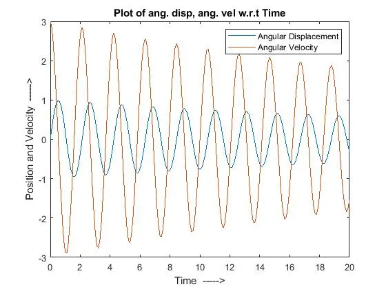
plot(t,results(:,1));
hold on
plot(t,results(:,2));
ylabel('Position and Velocity ----->');
xlabel('Time ----->');
title('Plot of ang. disp, ang. vel w.r.t Time');
legend('Angular Displacement','Angular Velocity');
x0=0;
y0=0;
ct=1; %counter actually represents each and every frame
for i=1:length(t_span)
x1=l*sin(results(i,1));
y1=-l*cos(results(i,1));
figure(2)
plot([-1 1],[0 0],'linewidth',6,'color','g');
axis([-2 2 -2 2]);
line([x0 x1],[y0 y1],'linewidth',2,'color','b');
hold on
plot(x0,y0,'o','markersize',3,'markerfacecolor','y','markeredgecolor','y');
plot(x1,y1,'o','markersize',20,'markerfacecolor','r','markeredgecolor','r');
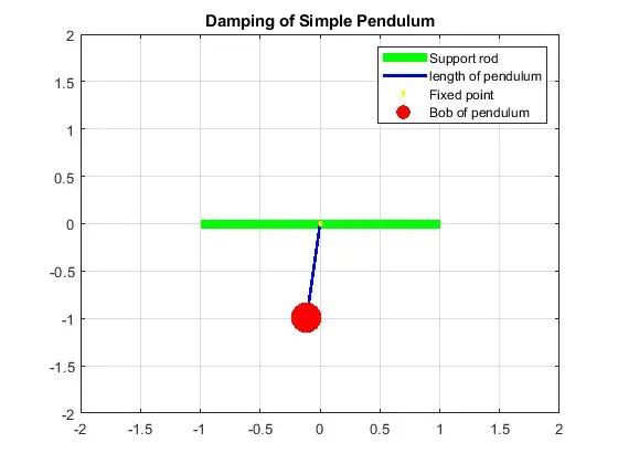
title('Damping of Simple Pendulum');
legend('Support rod','length of pendulum','Fixed point','Bob of pendulum');
grid on; %for noticing better bob's movements wrt grid locations as time proceeds
hold off %else the trace of bob will occur like a semicircular arc
pause(0.03) %pause is used to control the speed of animation moving
%for animation
M(ct)=getframe(gcf);
ct=ct+1;
end
%to make it into a video
movie(M)
videofile=VideoWriter('simple_pendulum.avi','Uncompressed AVI');
open(videofile)
writeVideo(videofile,M)
close(videofile)
%function used
function[dtheta_dt]=ode_func(t,theta,b,g,l,m)
theta1=theta(1);
theta2=theta(2);
dtheta1_dt=theta2; %first ODE
dtheta2_dt=-(b/m)*theta2-(g/l)*sin(theta1); %second ODE
dtheta_dt=[dtheta1_dt;dtheta2_dt]; %combining both of ODEs into an array
end
EXPLANATION :
We can infer that the animation/video is more smooth/continous due to low damping coefficient, if damping coefficient is increased then, the resistance to the motion will be higher.
OUTPUT :
http://asciimath.org/#syntax https://drive.google.com/file/d/1aVCGMcnbyyclfy_MKvlEXn5Oq61cXb3g/view?usp=shari