Week 4 - Genetic Algorithm

AIM : To create and optimize stalagmite function  and to find the global maxima of function

THEORY : Genetic algorithm is an optimization technique which is used to minimise a certain function,when used in optimization ,generally its purpose to minimise the error of a function.This algorithm is named 'Genetic, because of its structure.It is a fittest of the survival algorithm.It incorporates the techniques of selection,  mutation, inheritance, recombination. 'ga' is also  inbuilt function in matlab,which is used to find the minimum value.

CODE : 

%main program
clear all
close all
clc

%defining our search space
x=linspace(0,0.6,150);
y=linspace(0,0.6,150);

%creating a 2Dimensional mesh
[xx,yy]=meshgrid(x,y);
n=length(x); %defines the length of x or y or xx or yy as all are of equal length
f=zeros(n,n); %preallocating the size of matrix to increase performance speed
%evaluating the stalagmite function
for i=1:length(x)
for j=1:length(y)
input_vector(1)=xx(i,j);
input_vector(2)=yy(i,j);
f(i,j)=stalagmite(input_vector);%function calling and the value is
% also assigned to LHS
end
end

iterations=100;
%preallocating the matrices so that their size is created beforehand,during
%iterations matlab only rewrites values, this process is less time
%consuming than recreating the size each time of iteration
fval1=zeros(1,iterations);
fval2=zeros(1,iterations);
fval3=zeros(1,iterations);
x1=zeros(1,iterations);
x2=zeros(1,iterations);
x3=zeros(1,iterations);
y1=zeros(1,iterations);
y2=zeros(1,iterations);
y3=zeros(1,iterations);
%case 1 unbounded values
tic %time counter used for measuring time taken while executing specific part of script
for i=1:iterations %ga is genetic algorithm is an inbuilt function
[inputa,fval1(i)]=ga(@stalagmite,2);
x1(i)=inputa(1);
y1(i)=inputa(2);
clc %used to create
end
study_time1=toc; %time counter ends
%plotting
figure(1)
subplot(2,1,1) %used to have multipe plots in same figure-window
hold on
surfc(x,y,f)
shading interp %used as shading pattern instead of meshgrid, for better visualization
xlabel('X-values');
ylabel('Y-values');
plot3(x1,y1,fval1,'marker','o','markersize',4,'markerfacecolor','r'); %used to make 3D plot
title 'Case 1: Unbounded values';
legend ('Function','Minima');
subplot(2,1,2)
plot(fval1)
xlabel('Iterations');
ylabel('Function Minimum');
title('Minimum value at different iterations');

%bounding the value of x
tic
for i=1:iterations
[inputb,fval2(i)]=ga(@stalagmite,2,[],[],[],[],[0;0],[1;1]);
x2(i)=inputb(1);
y2(i)=inputb(2);
clc
end
study_time2=toc;

%plotting

figure(2)
subplot(2,1,1)
hold on
surfc(x,y,f)
shading interp
xlabel('X-values');
ylabel('Y-values');
plot3(x2,y2,fval2,'marker','o','markersize',4,'markerfacecolor','r');
title 'Case 2: Bounded values';
legend ('Function','Minima');
subplot(2,1,2)
plot(fval2)
xlabel('Iterations');
ylabel('Function Minimum');
title('Minimum value at different iterations');

%case 3(Bounding values and also increasing population by 400)
options=optimoptions('ga');
options=optimoptions(options,'populationsize',400);

tic
for i=1:iterations
[inputc,fval3(i)]=ga(@stalagmite,2,[],[],[],[],[0;0],[1;1],[],[],options);
x3(i)=inputc(1);
y3(i)=inputc(2);
clc
end
study_time3=toc;

%plotting

figure(3)
subplot(2,1,1)
hold on
surfc(x,y,f)
shading interp
xlabel('X-values');
ylabel('Y-values');
plot3(x3,y3,fval3,'marker','o','markersize',4,'markerfacecolor','r');
title 'Case 3: Bounded values with increased population';
legend ('Function','Minima');
subplot(2,1,2)
plot(fval3)
xlabel('Iterations');
ylabel('Function Minimum');
title('Minimum value at different iterations') ;

%how actually a stalagmite looks in nature
figure(4)
hold on
surf(x,y,-f) %note the change in f and also from surf to surfc
shading interp
xlabel('X-values');
ylabel('Y-values');
plot3(x3,y3,-fval3,'marker','o','markersize',4,'markerfacecolor','r');
title 'Stalagmite shape found in Nature';
legend ('Function','Maxima');
colorbar
%to display time, also num2tr converts numerical array into character array
%that represents numbers
A=['The study time for case 1: will be ',num2str(study_time1),' seconds']
B=['The study time for case 2: will be ',num2str(study_time2),' seconds']
C=['The study time for case 3: will be ',num2str(study_time3),' seconds']

%function used in ga_main2 program

function[F]=stalagmite(input_vector)
%function that creates a stalagmite function with base equations
x=input_vector(1);
y=input_vector(2);
%the equation for a stalagmite function depends upon 2 variables x and y
%the formulae required for output is given below:
%f1a=(sin(5.1*pi*x+0.5))^6
%f1b=(sin(5.1*pi*y+0.5))^6
%f2a=exp(-4*log(2)*((x-0.0667)^2)/0.64)
%f2b=exp(-4*log(2)*((y-0.0667)^2)/0.64)

f1a=(sin(5.1*pi*x+0.5))^6;
f1b=(sin(5.1*pi*y+0.5))^6;
f2a=exp(-4*log(2)*((x-0.0667)^2)/0.64);
f2b=exp(-4*log(2)*((y-0.0667)^2)/0.64);

F=-1*(f1a*f1b*f2a*f2b);
end

OUTPUT : 

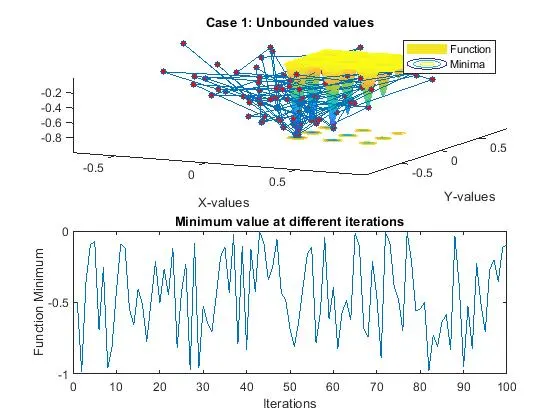
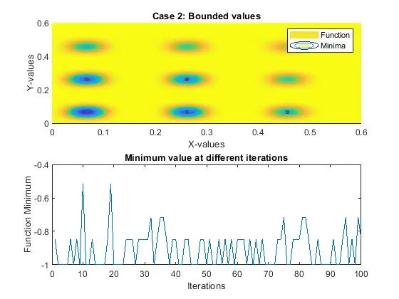
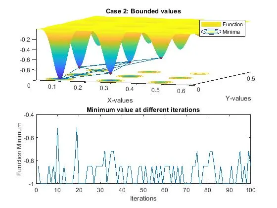
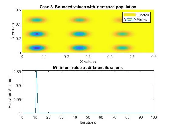
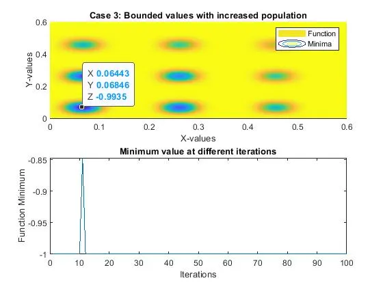
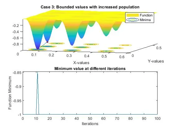
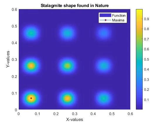
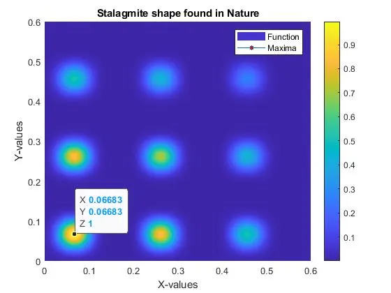
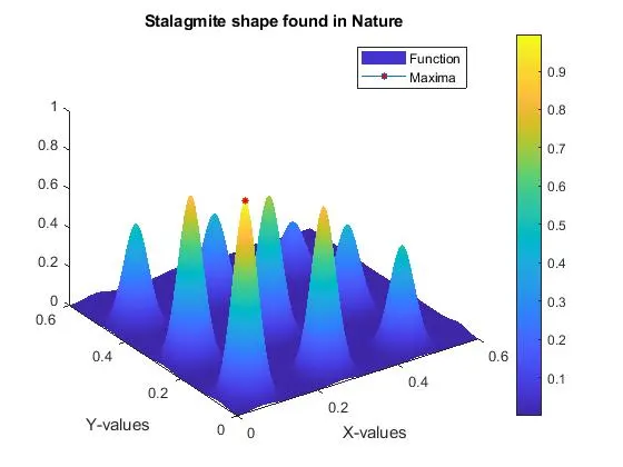
EXPLANATION : As the number of iterations and population size  increases, the time taken for the study also increases, but the chances of converging into a global maxima instead of a local maxima gets significantly higher.The value returned by ga is -1(global minima) always , except for 1 iteration where it is -0.85.The global maxima value happens to be at (0.06683,0.06683) of x,y coordinates where it is 1.

The studytime for case :1 is 7.9852 seconds , studytime for case :2 is 11.8422 seconds , finally studytime for case :3 is 65.8023 seconds.https://www.geeksforgeeks.org/genetic-algorithms/