Project 2 - Rankine cycle Simulator
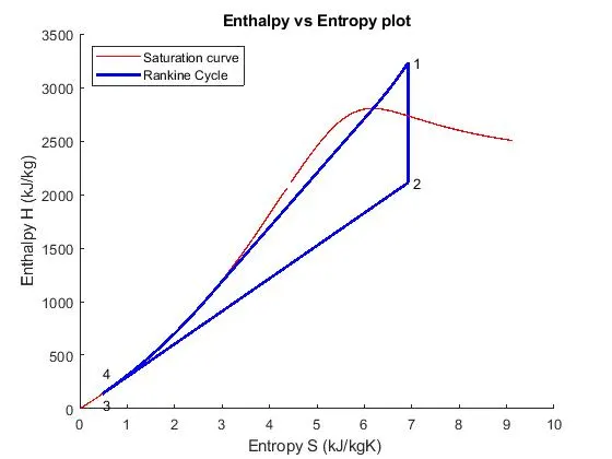
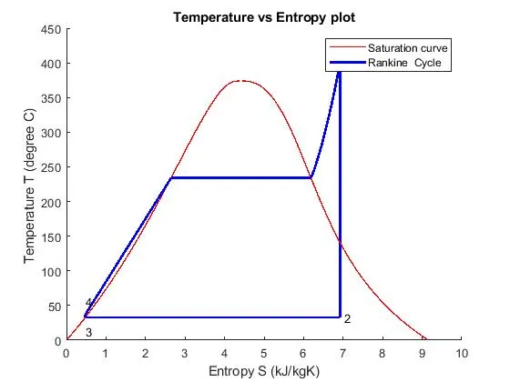
AIM: To create a Rankine Cycle Simulator using MATLAB and to calculate the state points of Rankine Cycle based on user inputs, also to calculate the net work output and back work ratio and finally to plot the T-s and h-s diagrams .
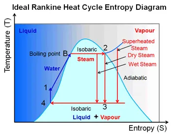
THEORY: The Rankine cycle is a model used to predict the performance of steam turbine systems. It was also used to study the performance of reciprocating steam engines. The Rankine cycle is an idealized thermodynamic cycle of a heat engine that converts heat into mechanical work while undergoing phase change. It is an idealized cycle in which friction losses in each of the four components are neglected. The heat is supplied externally to a closed loop, which usually uses water as the working fluid.
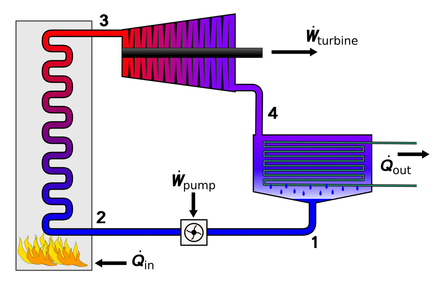
The are four processes in the rankine cycle are below:
- Process 1-2 : Isentropic Expansion in the turbine .
- Process 2-3 : Constant pressure Heat rejection in condenser
- Process 3-4 : Isentropic compression in the pump
- Process 4-1 : Constant pressure heat addition in the boiler
1. Turbine:
Isentropic expansion of the working fluid takes place in the turbine which results in work output. Thus, this process is work producing. The outlet of this process is mostly a mixture of liquid and vapour but it could be saturated vapour depending upon turbine inlet condition. The work produced in this process can be given as:
`W_(turb)=h_1-h_2`
2. Condenser:
In condensor, constant pressure heat rejection process convert all the vapour output of the turbine into saturated liquid. It is then entered into feed pump. The heat rejected in the process can be given as:
`q_(out)=h_2-h_3`
3. Feedpump:
Saturated liquid which is outcome of the condensor enters into pump which increases its pressure to the boiler pressure isentropically. This process is work consuming which is given as follows :
`W_(pump)=h_4-h_3`
4. Boiler:
In boiler, constant pressure heat addition process takes place which increases the enthalpy of the working fluid to sufficient value. The fluid could be heated upto saturated vapour state or could be superheated. The heat added to the working fluid in the boiler can be given as:
`q_i=h_1-h_4`
Here we have considered for idealized rankine cycle neglecting losses.
CODE:
%% Rankine Cycle Simulator
% Objective of this program is to simulate the rankine cycle
% Plotting t-s and h-s diagram using data from XSteam data
% Water and steam properties according to IAPWS IF-97
clear all
close all
clc
%%
disp(' RANKINE CYCLE SIMULATOR '); % Displaying
fprintf('\n');
disp('1-2 is Isentropic Expansion in the Turbine');
disp('2-3 is constant pressure heat rejection by the Condenser');
disp('3-4 is Isentropic compression in the Pump');
disp('4-1 is Constant pressure heat addition by the Boiler');
%%
%Obtaining the input data
p1 = input('\nEnter the Pressure at turbine inlet, p1(in bar) = ');
T1 = input('Enter the Temperature at turbine inlet, T1(in degree.C) = ');
p2 = input('Enter the Pressure at condenser inlet, p2(in bar) = ');
%%
% Extracting data _ defining variables
% State 1
% extracting enthalpy at state pt 1
h1 = XSteam('h_pT', p1, T1); %Entalpy as a function of pressure and temperature
% extracting entropy at state pt 1
s1 = XSteam('s_pT', p1, T1); %Specific entropy as a function of pressure and
%temperature (Returns saturated vapour entalpy if mixture
% State 2
s2 = s1; % Isentropic expansion
sf2= XSteam('sL_p', p2); % Saturated liquid Entropy
sg2 = XSteam('sV_p', p2); % Saturated Vapour Entropy
x2 = (s2-sf2)/(sg2-sf2); %x is dryness fraction
hf2 = XSteam('hL_p', p2); %Saturated liquid enthalpy
hg2 = XSteam('hV_p', p2); %Saturated vapour enthalpy
h2 = hf2 + (x2*(hg2-hf2));
% State 3
p3 = p2; % Constant pressure Heat rejection in condenser
s3= XSteam('sL_p', p3);
h3 = XSteam('hL_p', p3);
% State 4
s4 = s3; %since 3-4 is Isentropic compression in the Pump
p4 = p1; %since 4-1 is Constant pressure heat addition
%by the Boiler or we can say after 3-4 compression
%pressure is increased
%%
% Work done by turbine
Wt = h1 - h2;
% Work done to run pump
v3 = XSteam('vL_p', p3); %Saturated liquid volume
Wp = v3*(p4 - p3)*100;
h4 = h3 + Wp;
%net work
Wnet = Wt - Wp;
%backwork ratio
Back_Work_Ratio = Wp/Wt;
%Heat into the system
Qin = h1 - h4;
%Heat out of the system
Qout = h2 - h3;
%Thermal efficiency
eff = (Wnet/Qin)*100;
%Specific Steam Consumption
%SSC = mass flow rate/power
SSC = (3600/Wnet);
%%
%Calculating temperatures at the state points
T3 = XSteam('Tsat_p', p3); %Saturation temperature
T2 = T3;
Cp4 = XSteam('Cp_ps', p4, s4); %Specific isobaric heat capacity as a function
%of pressure and entropy
Cv4 = XSteam('Cv_ps', p4, s4); %Specific isobaric heat capacity as a function
%of pressure and entropy
k = Cp4/Cv4; %Specific heat ratio
T4 = T3/((p3/p4)^((k-1)/k)); %derived from isentropic relation
%Calculating temperature, entropy and enthalpy at the vapour and liquid
%line for plotting
T6 = XSteam('Tsat_p', p1);
s5 = XSteam('sL_p', p1);
s6 = XSteam('sV_p', p1);
h5 = XSteam('hL_p', p1);
h6 = XSteam('hV_p', p1);
T5 = T6;
%%
%Plotting the saturation curve
T = linspace(1,400,1500);
for i = 1:length(T)
sf(i) = XSteam('sL_T', T(i)); %Saturated liquid entropy
sg(i) = XSteam('sV_T', T(i)); %Saturated vapour entropy
hf(i) = XSteam('hL_T', T(i)); %Saturated liquid enthalpy
hg(i) = XSteam('hV_T', T(i)); %Saturated vapour enthalpy
end
%Plotting T-s diagram
figure(1)
hold on
plot(sf, T, 'r','linewidth',1)
plot([s1 s2], [T1 T2], 'b', 'linewidth', 2) %changing plot order for easy mapping of 2nd
%name in legends(Rankine Cycle)
plot(sg, T, 'r','linewidth',1)
plot([s2 s3], [T2 T3], 'b', 'linewidth', 2)
plot([s3 s4], [T3 T4], 'b', 'linewidth', 2)
plot([s4 s5], [T4 T5], 'b', 'linewidth', 2)
plot([s5 s6], [T5 T6], 'b', 'linewidth', 2)
sc1 = linspace(s6, s1, 1000);
for l = 1:length(sc1)
Tc1(l) = XSteam('T_ps', p1, sc1(l)); %Temperture as a function of pressure and entropy
end
plot(sc1, Tc1, 'b', 'linewidth', 2)
text(s1+0.1, T1, '1')
text(s2+0.1, T2, '2')
text(s3, T3-20, '3')
text(s4, T4+20, '4')
title('Temperature vs Entropy plot')
xlabel('Entropy S (kJ/kgK)')
ylabel('Temperature T (degree C) ')
legend('Saturation curve','Rankine Cycle')
%%
%Plotting h-s diagram
figure(2)
hold on
plot(sf, hf, 'r', 'linewidth', 1)
plot([s1 s2], [h1 h2], 'b', 'linewidth', 2)
plot(sg, hg, 'r', 'linewidth', 1)
plot([s2 s3], [h2 h3], 'b', 'linewidth', 2)
plot([s3 s4], [h3 h4], 'b', 'linewidth', 2)
hc = linspace(h4, h5, 100);
for k = 1:length(hc)
sch(k) = XSteam('s_ph', p1, hc(k)); %Specific entropy as a function of
%pressure and enthalpy
end
plot(sch,hc, 'b', 'linewidth', 2)
plot([s5 s6], [h5 h6], 'b', 'linewidth', 2)
for m = 1:length(sc1)
hc1(m) = XSteam('h_ps', p1, sc1(m)); % Entalpy as a function of pressure and entropy
end
plot(sc1, hc1, 'b', 'linewidth', 2)
text(s1+0.1, h1, '1')
text(s2+0.1, h2, '2')
text(s3, h3-100, '3')
text(s4, h4 +200, '4')
title('Enthalpy vs Entropy plot')
xlabel('Entropy S (kJ/kgK) ')
ylabel('Enthalpy H (kJ/kg)')
legend('Saturation curve','Rankine Cycle','location','northwest')
%%
% Displaying Results
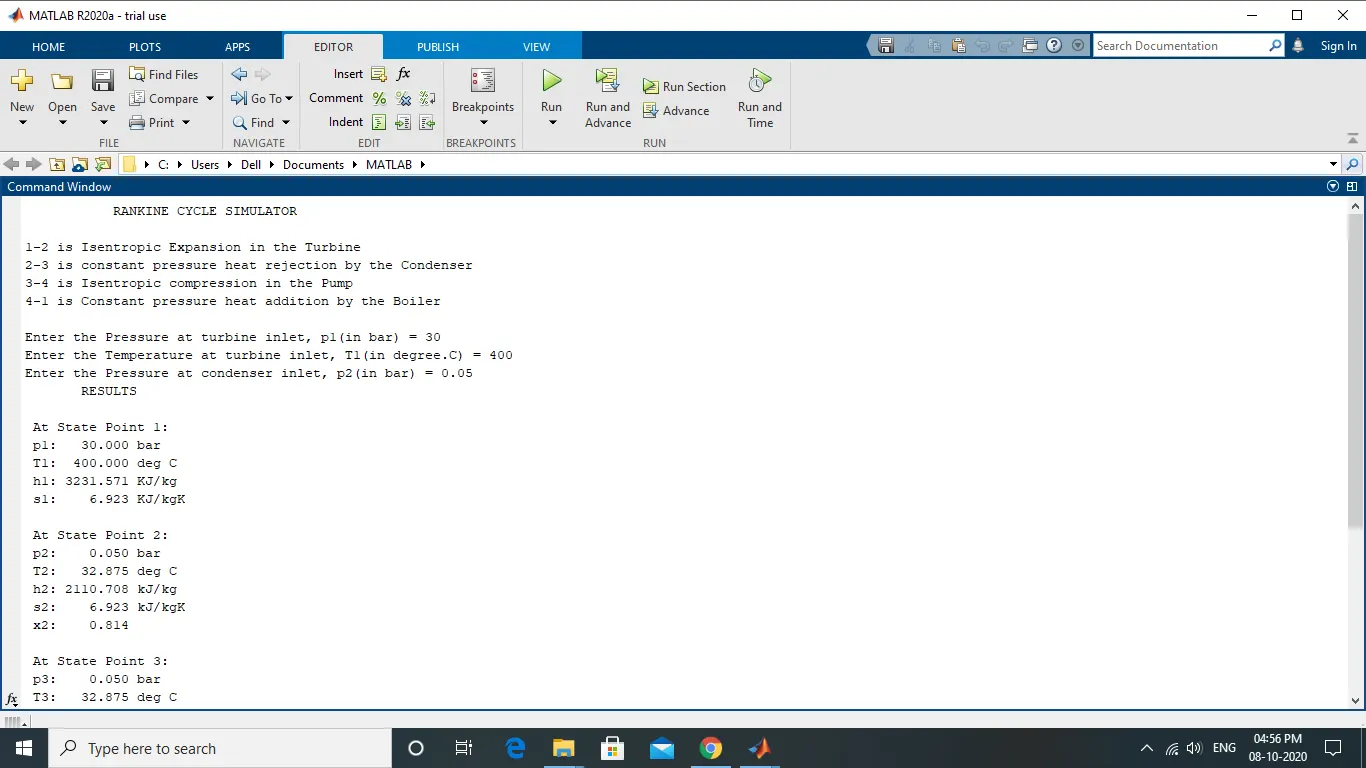
disp(' RESULTS');
fprintf('\n At State Point 1:');
fprintf('\n p1: %8.3f bar', p1);
fprintf('\n T1: %8.3f deg C', T1);
fprintf('\n h1: %8.3f KJ/kg', h1);
fprintf('\n s1: %8.3f KJ/kgK', s1);
fprintf('\n\n At State Point 2:');
fprintf('\n p2: %8.3f bar', p2);
fprintf('\n T2: %8.3f deg C', T2);
fprintf('\n h2: %8.3f kJ/kg', h2);
fprintf('\n s2: %8.3f kJ/kgK', s2);
fprintf('\n x2: %8.3f', x2);
fprintf('\n\n At State Point 3:');
fprintf('\n p3: %8.3f bar', p3);
fprintf('\n T3: %8.3f deg C', T3);
fprintf('\n h3: %8.3f kJ/kg', h3);
fprintf('\n s3: %8.3f kJ/kgK', s3);
fprintf('\n\n At State Point 4:');
fprintf('\n p4: %8.3f bar', p4);
fprintf('\n T4: %8.3f deg C', T4);
fprintf('\n h4: %8.3f kJ/kg', h4);
fprintf('\n s4: %8.3f kJ/kgK', s4);
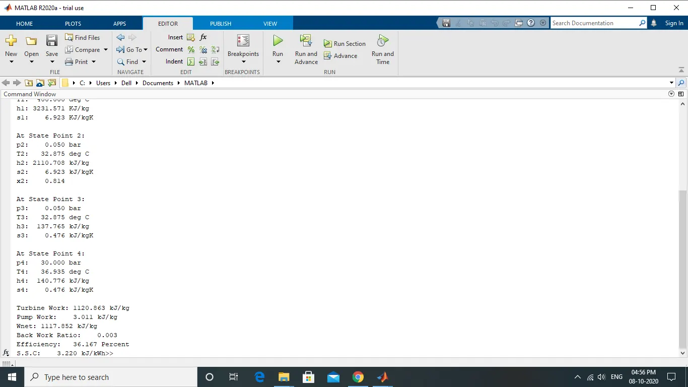
fprintf('\n\n Turbine Work: %8.3f kJ/kg', Wt);
fprintf('\n Pump Work: %8.3f kJ/kg', Wp);
fprintf('\n Wnet: %8.3f kJ/kg', Wnet);
fprintf('\n Back Work Ratio: %8.3f ',Back_Work_Ratio);
fprintf('\n Efficiency: %8.3f Percent ', eff);
fprintf('\n S.S.C: %8.3f kJ/kWh', SSC);
OUTPUT:
Note:
Even though the h-s plot's 4-1(blue) may look like a straight line, it consists of both curved and linear parts joined together. Also the attached rankine cycle numbering are different from the ones equations written for(it is corresponding to the code actually)