Week 3 - Taylor table method and Matlab code

AIM :

To write a program in Matlab to evaluate the second-order derivative of the analytical function exp(x)*cos(x) and compare it with the 3 numerical approximations that you have derived.

DESCRIPTION :

Taylor Table is a type of table which contains the data of all the Taylor series expansion of a function that can be used to calculate the analytical value of the higher-order derivative and plays an important role during numerical discretization. The more the terms we include, we are closer to the accurate results.

If the Numerical Stencils are not symmetric then we call that as Skewed 2nd order scheme.

Skewed Right-Sided Difference

`(del^2f)/(delx^2)=af_i+bf_(i+1)+cf_(i+2)+df_(i+3)+ef_(i+4)+gf(i+5)`

Term	`f(x)`	`Deltaxf'(x)`	`Deltax^2f''(x)`	`Deltax^3f'''(x)`	`Deltax^4f''''(x)`	`Deltax^5f'''''(x)`
af(i)	a	0	0	0	0	0
bf(i+1)	b	b	b/2	b/6	b/24	b/120
cf(i+2)	c	2c	4c/2	8c/6	16c/24	32c/120
df(i+3)	d	3d	9d/2	27d/6	81d/24	243d/120
ef(i+4)	e	4e	16e/2	64e/6	256e/24	1024e/120
gf(i+5)	g	5g	25g/2	125g/6	625g/24	3125g/120
`sum`	0	0	1	0	0	0

We should solve these 6 equations to get the value of a,b,c,d,e and f using matlab code.

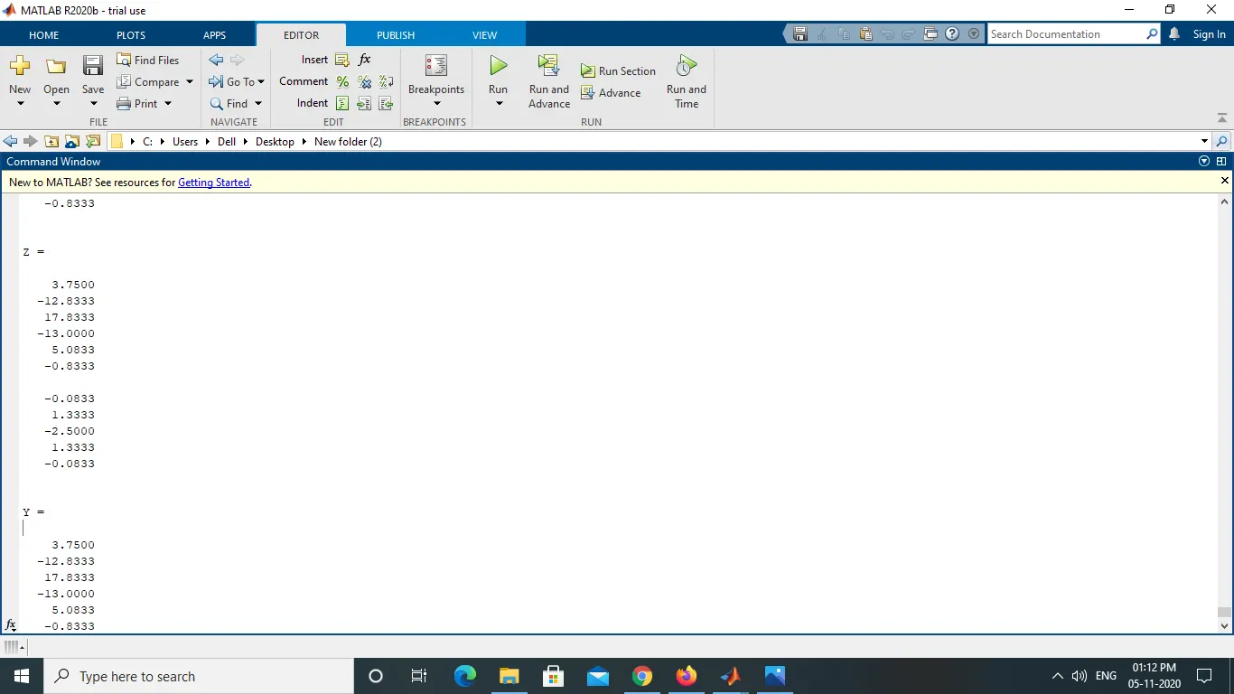
a=3.75, b=-12.8333, c=17.8333, d=-13, e=5.0833, g=-0.8333

Skewed Left-Sided Difference

`(del^2f)/(delx^2)=af_i+bf_(i-1)+cf_(i-2)+df_(i-3)+ef_(i-4)+gf_(i-5)`

Term	`f(x)`	`Deltaxf'(x)`	`Deltax^2f''(x)`	`Deltax^3f'''(x)`	`Deltax^4f''''(x)`	``Deltax^5f'''''(x)``
af(i)	a	0	0	0	0	0
bf(i-1)	b	-b	b/2	-b/6	b/24	-b/120
cf(i-2)	c	-2c	4c/2	-8c/6	16c/24	-32c/120
df(i-3)	d	-3d	9d/2	-27d/6	81d/24	-243d/120
ef(i-4)	e	-4e	16e/2	-64e/6	256e/24	-1024e/120
gf(i-5)	g	-5g	25g/2	-125g/6	625g/24	-3125g/120
`sum`	0	0	1	0	0	0

We should solve these 6 equations to get corresponding the value of a,b,c,d,e and f using matlab code.

a=3.75, b=-12.8333, c=17.8333, d=-13, e=5.0833, g=-0.8333

Central Difference Scheme

`(del^2f)/(delx^2)=af_(i-2)+bf_(i-1)+cf_(i)+df_(i+1)+ef_(i+2)`

Term	`f(x)`	`Deltaxf'(x)`	`Deltax^2f''(x)`	`Deltax^3f'''(x)`	`Deltax^4f''''(x)`
af(i-2)	a	-2a	4a/2	-8a/6	16a/24
bf(i-1)	b	-b	b/2	-b/6	b/24
cf(i)	c	0	0	0	0
df(i+1)	d	d	d/2	d/6	d/24
ef(i+2)	e	2e	4e/2	8e/6	16e/24
`sum`	0	0	1	0	0

We should solve these 5 equations to get corresponding the value of a,b,c,d,e using matlab code.

CODE :

clear all
close all
clc
%%
%main program
% Input variables
x = pi/3;
dx = linspace(pi/4,pi/4000,200);

for i = 1:length(dx)
 central_diff_value(i) = central_diff(x,dx(i)); 
 skewed_right_value(i) = skewed_right_diff(x,dx(i));
 skewed_left_value(i) = skewed_left_diff(x,dx(i));
end
figure(1)
loglog(dx,central_diff_value,'r')
hold on
loglog(dx,skewed_right_value,'b')
loglog(dx,skewed_left_value,'g')
hold off
title('Scheme Error Comparison')
legend('Central Differencing','Skewed Right','Skewed Left');
xlabel('Dx')
ylabel('Absolute Error')
%%

function error_CD = central_diff(x,dx)
 
%Central_Difference_Scheme
[A]=[1 1 1 1 1;-2 -1 0 1 2;2 1/2 0 1/2 2;-8/6 -1/6 0 1/6 8/6;16/24 1/24 0 1/24 16/24];
[B]=[0;0;1;0;0];

X=linsolve(A,B);
disp(X);

 % Given function 
 %f(x) = exp(x)*cos(x)
 % Second order derivative of the function
 second_order_derivative = -2*exp(x)*sin(x);
 
 % Calculating the central difference value 
 central_difference = ((-0.083333333333334)*(exp(x-(2*dx))*cos(x-(2*dx)))+(1.333333333333334)*(exp(x-(1*dx))*cos(x-(1*dx)))+(-2.500000000000001)*(exp(x)*cos(x))+(1.333333333333334)*(exp(x+(1*dx))*cos(x+(1*dx)))+(-0.083333333333334)*(exp(x+(2*dx))*cos(x+(2*dx))))/(dx^2); 
 %Error calculation 
 error_CD = abs(second_order_derivative - central_difference);
end
%%

function error_SR = skewed_right_diff(x,dx)

%Skewed Right Sided Scheme
C=[1 1 1 1 1 1;0 1 2 3 4 5;0 0.5 2 4.5 8 12.5;0 1/6 4/3 4.5 32/3 125/6;0 1/24 2/3 27/8 32/3 625/24;0 1/120 32/120 243/120 1024/120 3125/120];
[D]=[0;0;1;0;0;0];
P=inv(C);
Y=P*D;

disp(Y);

 % Given function 
 %f(x) = exp(x)*cos(x)
 % second order derivative of the function
 second_order_derivative = -2*exp(x)*sin(x);
 % calculating skewed right difference value 
 skewed_right_difference = (((Y(1))*(exp(x))*(cos(x)))+((Y(2))*(exp(x+(1*dx)))*cos(x+(1*dx)))+((Y(3))*(exp(x+(2*dx)))*cos(x+(2*dx)))+((Y(4))*(exp(x+(3*dx)))*cos(x+(3*dx)))+((Y(5))*(exp(x+(4*dx)))*cos(x+(4*dx)))+((Y(6))*(exp(x+(5*dx)))*cos(x+(5*dx))))/(dx^2);
 
 %Error calculation 
 error_SR = abs(second_order_derivative - skewed_right_difference);
end
%%

function error_SL = skewed_left_diff(x,dx)
 
%Skewed Left Sided Scheme
[E]=[1 1 1 1 1 1;0 -1 -2 -3 -4 -5;0 1/2 2 9/2 8 25/2;0 -1/6 -4/3 -9/2 -32/3 -125/6;0 1/24 2/3 27/8 32/3 625/24;0 -1/120 -32/120 -243/120 -1024/120 -3125/120];
[F]=[0;0;1;0;0;0];

Q=inv(E);
Z=Q*F;

disp(Z);

 % Given function 
 %f(x) = exp(x)*cos(x)
 % second order derivative of the function
 second_order_derivative = -2*exp(x)*sin(x);
 
 % Calculating the skewed left difference value 
 skewed_left_difference = (((Z(1))*(exp(x))*(cos(x)))+((Z(2))*(exp(x-(1*dx)))*cos(x-(1*dx)))+((Z(3))*(exp(x-(2*dx)))*cos(x-(2*dx)))+((Z(4))*(exp(x-(3*dx)))*cos(x-(3*dx)))+((Z(5))*(exp(x-(4*dx)))*cos(x-(4*dx)))+((Z(6))*(exp(x-(5*dx)))*cos(x-(5*dx))))/(dx^2);
 %Error calculation 
 error_SL = abs(second_order_derivative - skewed_left_difference);
end
%%

clear all
close all
clc
%%
%program to compare forward and backward differencing scheme

%taylor Table test
%analytical function f'=exp(x)*cos(x)
%f''=-2exp(x)*sin(x)

x=pi/3;
dx=linspace(pi/40,pi/4000,200);
analytical_function=exp(x)*cos(x);
analytical_der=-2*exp(x)*sin(x);

for i=1:length(dx);
    bd(i)=(exp(x)*cos(x)-exp(x-dx(i))*cos(x-dx(i)))/dx(i);
    fd(i)=(exp(x+dx(i))*cos(x+dx(i))-exp(x)*cos(x))/dx(i);
    br(i)=abs(bd(i)-analytical_der);
    fr(i)=abs(fd(i)-analytical_der);
end

figure(1)
loglog(dx,br,'r')
hold on
loglog(dx,fr,'b')
hold on
legend('Backward Error','Forward Error')
xlabel('dx')
ylabel('Error')
title('Forward Differencing & Backward Differencing Scheme Error Comparison')

OUTPUT :

INFERENCE :

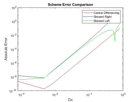
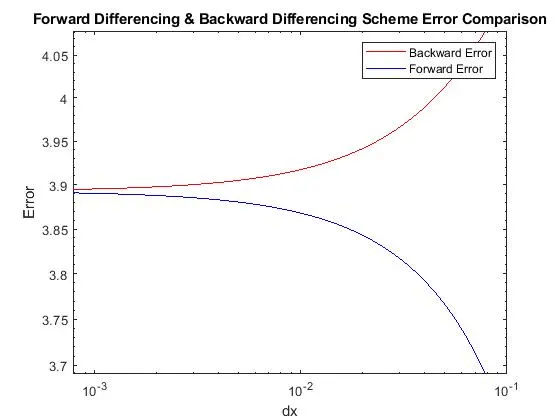
From the comparison of different schemes for 4th order approximation , we we can see that central difference approximation yields more accurate solution than both right and left skewed approximation schemes. Also from the other graph we can also deduce that since both forward and backward approximations are of second-order error, they give out larger errors than the other fourth-order schemes.

Reason for Skewed scheme usefulness is because ,since a function is always characterized by a domain. A domain is a space or area beyond which a function ceases to exist. Therefore a domain has boundaries and the function exists on only one side of the boundary. So, if we want to compute a numerical approximation for the function at the boundary, we cannot use a central difference scheme as it requires data from both sides of the boundary. This iswhy a skewed difference scheme plays a vital role since data from any side can be used to perform numerical approximation at a point.