Week 3 - Solving second order ODEs

AIM:

To write a python program that represents the(ODE) equation of motion of a simple pendulum with damping.

THEORY:

The second-order ODE is simple pendulum's harmonic motion with damper, hence with decreasing amplitude.

`(d^2theta)/(dt^2)+(b/m)*((d theta)/(dt))+(g/L)*sin(theta)=0`

This system is equivalent to mass attached with spring and damper. Generally, higher-order ODEs are solved by breaking them into single-order ODE. This is applicable in our case also.

`(d theta_1)/dt=theta_2`

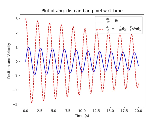
`(d theta_2)/dt=-(b/m)*theta_2-(g/L)*sintheta_1`

These are the 2 equations we get here

CODE:

import numpy as np
from scipy.integrate import odeint
import matplotlib.pyplot as plt
import math

# function that returns dz/dt
def model(theta,t,b,g,l,m):

	theta1=theta[0]
	theta2=theta[1]
	dtheta1_dt=theta2
	dtheta2_dt=-(b/m)*theta2-(g/l)*math.sin(theta1)
	dtheta_dt=[dtheta1_dt,dtheta2_dt]
	return dtheta_dt


b=0.05
g=9.81
l=1
m=1

#initial condition
theta_0=[0,3]

#time points
t=np.linspace(0,20,200)

#solve ODE
theta=odeint(model,theta_0,t,args=(b,g,l,m))

#plot results
plt.plot(t,theta[:,0],'b-',label=r'$\frac{d\theta_1}{dt}=\theta_2$')
plt.plot(t,theta[:,1],'r--',label=r'$\frac{d\theta_2}{dt}=-\frac{b}{m}\theta_2-\frac{g}{L}sin\theta_1$')
plt.xlabel('Time (s)')
plt.ylabel('Position and Velocity')
plt.title("Plot of ang. disp and ang. vel w.r.t time")
plt.legend(loc='best')
#plt.show()


x = theta[:,0]

ct = 1

# the for loop has been created because to show that the pendulum has run for 20 sec for different values of theta. 

for i in x:
    x0 = 0
    y0 = 0

    x1 =  (x0 + l*math.sin(i))
    y1 = -(y0 + l*math.cos(i))

    # plot function

    plt.figure()
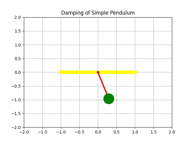
    plt.plot([-1 ,1] , [0,0] , color = "yellow" , linewidth = 8)
    plt.plot(x0,y0 , 'o' ,marker = 'o', markersize = 5  , color = "purple")
    plt.plot([ x0,x1] , [y0, y1] , linewidth = 3 , color = "red")
    plt.plot( x1 ,y1 , 'o' ,marker = 'o', markersize = 25  , color = "green")
    plt.title("Damping of Simple Pendulum")
    plt.xlim([-2,2])
    plt.ylim([-2,2])
    plt.grid ('on')
    filename = 'test%05d.png'  % ct # name for saving the filename to create image one by one
    #filename=str(ct)+'.png'
    plt.savefig(filename)
    ct =ct +1
    plt.show()

EXPLANATION:

We can infer that the animation/video is more smooth/continuous due to the low damping coefficient, if the damping coefficient is increased then, the resistance to the motion will be higher.

OUTPUT:

LINK: https://drive.google.com/file/d/18e2g5cbwN-kzjBv7g4p0_fCObnNC_iml/view?usp=sharing

Animation GIF has been created using the ImageMagick software.