Week 5 - Curve fitting

AIM :

To write a code in Python to fit a linear and cubic order polynomial for the given Cp data.

THEORY : Curve fitting is the process of constructing a curve or mathematical function that has the best fit to a series of data points, possibly subject to constraints or it can be defined as the process of finding an approximate mathematical model that expresses the relationship between a dependant variable y and a single independent variable x and estimating the values of its parameters using non-linear regression.

Questions:

1.'popt' represents the matrix that stores and extracts the coefficients for the fitting functions according to the general equations defined.

'pcov' represents the square matrix that stores the estimated values of covariance of the coefficients of the above. The diagonal elements of this square matrix also represent the variance of that coefficients.

2. This command converts each value of temperature in the data file into an array using numpy module.

3. The * here means that it is being referenced. Any and all change that could have occurred to popt while in a function would be reflected in the original popt.

4. A curve fit is said to be good when it's `R^2` value is `ge 0.95` in which case it's called as best fit.

5. When `R^2=1`, it's called a perfect fit. A curve fit can be almost perfect, but not 100% perfect. Some methods are

• By trying different order equations
• Splitting the data and curve fitting them separately.

CODE :

# Comparison of Linear and Cubic curve fit

import numpy as np
import matplotlib.pyplot as plt
from scipy.optimize import curve_fit

#Linear Curve fit function 
def func_linear(t,a,b):
	return a*t+b

#Cubic Curve fit function 
def func_cubic(t,a,b,c,d):
	return a*pow(t,3)+b*pow(t,2)+c*t+d


# Reading thermodynamic data file
def read_file():
	temperature=[]
	cp=[]
	for line in open('data','r'):
		values=line.split(',')
		temperature.append(float(values[0]))
		cp.append(float(values[1]))

	return [temperature,cp]

#Main program

temperature,cp=read_file()
popt_1,pcov_1=curve_fit(func_linear,temperature,cp)  #popt contains the 2 unknowns a,b
fit_cp_linear=func_linear(np.array(temperature),*popt_1)  #using a '*' helps us to refer these values  , fit_cp is  like predicted_cp

popt_3,pcov_3=curve_fit(func_cubic,temperature,cp)  #popt contains the 4 unknowns a,b,c and d
fit_cp_cubic=func_cubic(np.array(temperature),*popt_3)

plt.plot(temperature,cp,color="blue",linewidth=3)
plt.plot(temperature,fit_cp_linear,color="red",linewidth=3)
plt.plot(temperature,fit_cp_cubic,color="green",linewidth=3)
plt.title("Curve fit")
plt.grid ('on')
plt.legend(['Original dataset','Linear fit','Cubic fit'])
plt.xlabel('Temperature [k]')
plt.ylabel('Specific heat    (Cp)')
plt.savefig('Curve fit')

plt.show()

OUTPUT :

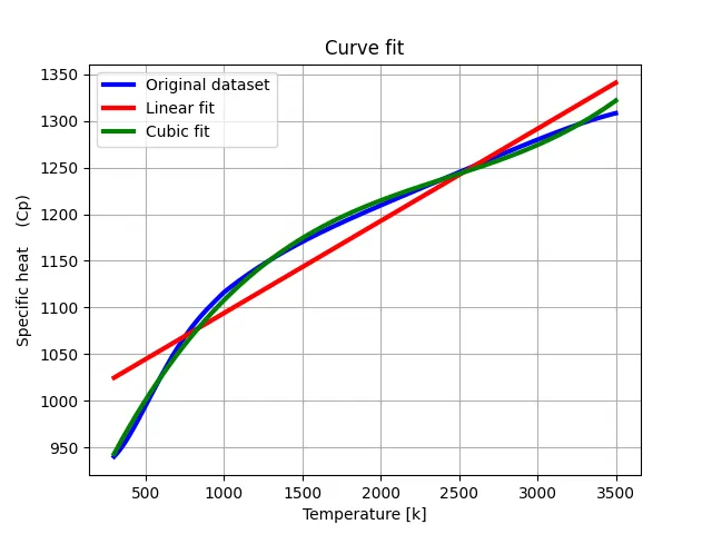
CONCLUSION :

It can be inferred that as the degree of polynomial increases, the curve fit tends to exactly match the original data. Also, we can easily this nature in linear and cubic curve fit.