Week 3 - Solving second order ODEs

Solving second order ODEs

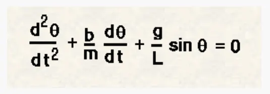
PROGRAM TO SOLVE THE FOLLOWING ODE

CODE;

%PROGRAM TO SOLVE THE FOLLOWING ODE
close all
clear all
clc

%Inputs
b = 0.05;
g = 9.81;
l = 1;
m = 1;

%Initial condition
theta_0 = [0;3];

%Time points
t_span = linspace (0,20,350);

%solve ODE
[t, results] = ode45(@(t,theta) ode_funs(t,theta,b,g,l,m),t_span,theta_0);

%Plotting B\W displacement and velocity

%for figure 1

plot(t,results(:,1))
hold on
plot(t,results(:,2))
xlabel('Time')
ylabel('Plot')
legend('Angular displacement','Angular velocity')

%for loop to make the animation

ct = 1;
for i = 1:length(results(:,1))
    x0 = 0;
    y0 = 0;
    
    x1 = l*sin(results(i,1));
    y1 = -l*cos(results(i,1));
    % Plotting the animation
    figure(2)
    plot([-1 1],[0 0],'linewidth',17,'Color','#7E2F8E')
    hold on
    plot([x0 x1],[y0 y1],'linewidth',4,'Color','#A2142F')
    hold on
    plot(x1,y1,'o','markersize',20,'markerfacecolor','k')
    axis([-2 2 -2 2])
    pause(0.03)
    hold off
    M(ct) = getframe(gcf);
    ct = ct+1;
end




% To Convert the animation into a movie
movie(M)
videofile = VideoWriter('pendulum_oscillation.avi','Uncompressed AVI');
open(videofile)
writeVideo(videofile,M)
close(videofile)

FUNCTION CODE

%DEFINING ODE function 
function [dtheta_dt] = ode_funs(t,theta,b,g,l,m)

        theta1 = theta(1)
        theta2 = theta(2)
        dtheta1_dt = theta2;
        dtheta2_dt = -(b/m)*theta2 - (g/l)*sin(theta1);
        dtheta_dt = [dtheta1_dt ; dtheta2_dt];
end

CODE EXPLANATION;

• The angular displacement is initillay set at 0 & the angular velocity is set as 3

• Time span is taken in linspace command from 0-20 in 600 values

• Function is defined based on the derivation to split the 2nd Order Differential Equation into two 1st Order Differential Equation. Once θ1 and θ2 are defined, they are stored as a solution vector

• where, dtheta_dt = [dtheta1_dt ; dtheta2_dt]; is a column matrix.

• ODE 45 is inbuilt command in matlab to solve the second order differential equation.

• @(t,theta) is the input argument of the anonymous function and ode_func(t,theta,b,g,l,m),t_span,theta_0 is the definition of the anonymous function.

• Function must be defined for solving the ode by considering different parameters such as time span,theta,damping coefficient,gravity,length,mass of the pendulum.

• In this program function is named as ode_funs to call the function to calculate the ode of pendulum.

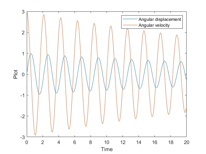
• The graph between the velocity and displacemet using the plot command.

• For loop is used to asign the iterations and to perform the program untill it reaches the maximum iteration levels.

• counter command is used to increase the iteration in the defined order.

• Marker command plays the vital role in this problem to create the pendulum.

• The color comand is used to colour the various part of the pendulum.

• hold off sets the hold state to off so that new plots added to the axes clear existing plots and reset all axes properties.

• To convert the animation into video video file and video write command is used.

PLOTTINGS

VIDEO LINK FOR THE PENDULUM ODE

https://youtu.be/5W94dXFQjFc