Week 3 - Adiabatic Flame Temperature calculation
Objective
To calculate adiabatic flame temperature for different cases in python and cantera.
Adiabatic flame temperature (AFT)
In the study of combustion, there are two types of adiabatic flame temperature depending on how the process is completed: the constant volume and constant pressure.
The constant volume adiabatic flame temperature is the temperature that results from a complete combustion process that occurs without any work, heat transfer or changes in kinetic or potential energy. Its temperature is higher than the constant pressure process because no energy is utilized to change the volume of the system.
Equivalence ratio
It is the ratio of fuel concentration in the actual fuel-air mixture divided by the fuel concentration in a stoichiometric mixture.
If Equivalence ratio = 1, then it is stoichiometric mixture
If Equivalence ratio > 1, then it is rich mixture
If Equivalence ratio < 1, then it is lean mixture
Case 1: Adiabatic flame temperature variation with Equivalence ratio (In constant volume-chamber) :
The stoichiometric combustion of the methane is as follows :

For lean mixture, the reaction is as follows :

For rich mixture, the reaction is as follows :

The enthalpies are calculated with the help of the polynomial function provided by NASA for a particular temperature.
For constant volume condition, the enthalpy equation will be as follows :

Newton Raphson method is used to solve the enthalpy equation since it is a polynomial function. This method is used to find the roots of the equation using an initial guess value and iterate till we reach the given tolerance value. The equation is given by :
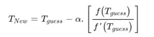
where,
Tnew is the calculated new temperature.
Tguess is the initial guess value of temperature.
α is the relaxation factor and its value is taken as 0.2.
The program for Python and Cantera is given below :
"""
program for different values of AFT of methane at different equivalence ratios

Stoichometric Reaction
CH4 + 2(O2+3.76N2) = CO2 + 2H2O + 7.52N2
Lean mixture (fi < 1)
CH4 + 2/fi*(O2+3.76N2) = CO2 + 2H2O+ (2/fi - 2)*O2 + 7.52/fi*N2
Rich Mixture (fi > 1)
CH4 + 2/fi*(O2+3.76N2) = (4/fi - 3)*CO2 + 2H20 + (4-4/fi)*CO + 7.52/fi*N2
"""

import cantera as ct
import matplotlib.pyplot as plt
import math
import numpy as np

def h(T, coeffs):
	# Function to evaluate enthalpy

	R = 8.314 #J/mol-K,kJ/kmol-K
	a1 = coeffs[0]
	a2 = coeffs[1]
	a3 = coeffs[2]
	a4 = coeffs[3]
	a5 = coeffs[4]
	a6 = coeffs[5]

	return (a1 + a2*T/2 + a3*pow(T,2)/3 + a4*pow(T,3)/4 + a5*pow(T,4)/5 + a6/T)*R*T

# Low temperatue coefficients
ch4_coeffs_l = [5.14987613E+00,-1.36709788E-02,4.91800599E-05,-4.84743026E-08,1.66693956E-11,-1.02466476E+04,-4.64130376E+00]

o2_coeffs_l = [3.78245636E+00,-2.99673416E-03,9.84730201E-06,-9.68129509E-09,3.24372837E-12,-1.06394356E+03,3.65767573E+00]

n2_coeffs_l = [0.03298677E+02,0.14082404E-02,-0.03963222E-04,0.05641515E-07,-0.02444854E-10,-0.10208999E+04,0.03950372E+02]

# High temperatue coefficients

o2_coeffs_h = [3.28253784E+00,1.48308754E-03,-7.57966669E-07,2.09470555E-10,-2.16717794E-14,-1.08845772E+03,5.45323129E+00]

n2_coeffs_h = [0.02926640E+02,0.14879768E-02,-0.05684760E-05,0.10097038E-09,-0.06753351E-13,-0.09227977E+04,0.05980528E+02]

co2_coeffs_h = [3.85746029E+00,4.41437026E-03,-2.21481404E-06,5.23490188E-10,-4.72084164E-14,-4.87591660E+04,2.27163806E+00]

h2o_coeffs_h = [3.03399249E+00,2.17691804E-03,-1.64072518E-07,-9.70419870E-11,1.68200992E-14,-3.00042971E+04, 4.96677010E+00]

co_coeffs_h = [2.71518561E+00,2.06252743E-03,-9.98825771E-07,2.30053008E-10,-2.03647716E-14,-1.41518724E+04,7.81868772E+00]

def f(T, fi):
# function that represents the root finding problem

	h_co2_p = h(T,co2_coeffs_h)
	h_n2_p = h(T,n2_coeffs_h)
	h_h2o_p = h(T,h2o_coeffs_h)
	h_o2_p = h(T,o2_coeffs_h)
	h_co_p = h(T,co_coeffs_h)

	if fi > 1:

		H_products = (4/fi - 3)*h_co2_p + 2*h_h2o_p + (7.52/fi)*h_n2_p + (4 - 4/fi)*h_co_p
		n_products = ((4/fi - 3) + 2 + (7.52/fi) + (4 - 4/fi))

	if fi <= 1:

		H_products = h_co2_p + (7.52/fi)*h_n2_p + 2*h_h2o_p + ((2/fi) - 2)*h_o2_p
		n_products = (1 + ((2/fi)-2) + (7.52/fi) + 2)

	Tstd = 298.15
	R = 8.314 #J/mol-K

	h_ch4_r = h(Tstd,ch4_coeffs_l)
	h_o2_r = h(Tstd,o2_coeffs_l)
	h_n2_r = h(Tstd,n2_coeffs_l)

	H_reactants = h_ch4_r + (2/fi)*(h_o2_r + (3.76*h_n2_r))
	n_reactants = (1 + (2/fi) + (7.52/fi))

	return (H_products - H_reactants) - R*(n_products*T - n_reactants*Tstd)

def fprime(T,fi):
	return (f(T+1e-6,fi) - f(T, fi))/1e-6

T_guess = 1500
tol = 1e-4
alpha = 0.2

fi = np.linspace(0.1,2,20)

T_aft = []

for i in range(0, len(fi)):

	while abs(f(T_guess, fi[i])) > tol:
		T_guess = T_guess - alpha*((f(T_guess,fi[i]))/(fprime(T_guess,fi[i])))
	T_aft.append(T_guess)

print(T_aft)
gas = ct.Solution('gri30.xml')
aft = []

for i in range (0, len(fi)):
	n_total = (1 + (2/fi[i]) + (7.52/fi[i]))
	n_ch4 = 1/n_total
	n_o2 = (2/fi[i])/n_total
	n_n2 = (7.52/fi[i])/n_total
	gas.TPX = 298.15,101325,{'CH4':n_ch4, 'O2' :n_o2, 'N2' :n_n2}
	gas.equilibrate('UV','auto')
	aft.append(gas.T)

print(aft)

plt.plot(fi,T_aft,'-o', color = 'red', label = 'Python')
plt.plot(fi, aft,'-o', color = 'green', label = 'Cantera')
plt.legend()
plt.grid('on')
plt.xlabel("Equivalence Ratio")
plt.ylabel("Adiabatic Flame Temperature (K)")
plt.title("Variation of Adiabatic Flame Temperature with Equivalence Ratio")
plt.show()
The plot of variation of adiabatic flame temperature with equivalence ratio is shown below :
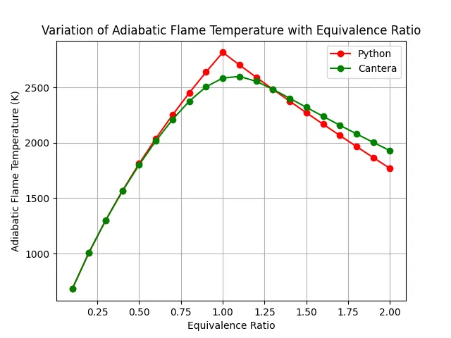
The highest AFT for python is found at Φ = 1 whereas the highest AFT for cantera is fouund at Φ > 1 (close to 1.1). The maximum AFT in case of python is 2817.83K (observed at Φ = 1) whereas the maximum AFT in case of cantera is around 2600.54K (observed at Φ > 1). The lower temperature in cantera as compared to python is due to the minimization of Gibbs free energy method used by cantera. Also the number of species formed in cantera are more which takes away the generated heat. This causes reduction of AFT in case of cantera.
Case 2. Adiabatic flame temperature variation with Heat loss (In constant pressure-chamber) :
In this case of constant pressure chamber, heat loss is considered thus the reaction is not going to be adiabatic. The heat loss factor is varied from no heat loss to entire heat loss. The enthalpy equation considering heat loss is as follows :

Python code
"""
stoichometric
CH4 + 2(O2+3.76N2) = CO2 + 2H2O + 7.52N2

For reactor at constant pressure condition, LHV= 50MJ

"""

import matplotlib.pyplot as plt
import math
import numpy as np

def h(T, coeffs):
	# Function to evaluate enthalpy

	R = 8.314 #J/mol-K,kJ/kmol-K
	a1 = coeffs[0]
	a2 = coeffs[1]
	a3 = coeffs[2]
	a4 = coeffs[3]
	a5 = coeffs[4]
	a6 = coeffs[5]

	return (a1 + a2*T/2 + a3*pow(T,2)/3 + a4*pow(T,3)/4 + a5*pow(T,4)/5 + a6/T)*R*T

ch4_coeffs_l = [5.14987613E+00,-1.36709788E-02,4.91800599E-05,-4.84743026E-08,1.66693956E-11,-1.02466476E+04,-4.64130376E+00]

o2_coeffs_l = [3.78245636E+00,-2.99673416E-03,9.84730201E-06,-9.68129509E-09,3.24372837E-12,-1.06394356E+03,3.65767573E+00]

n2_coeffs_l = [0.03298677E+02,0.14082404E-02,-0.03963222E-04,0.05641515E-07,-0.02444854E-10,-0.10208999E+04,0.03950372E+02]

n2_coeffs_h = [0.02926640E+02,0.14879768E-02,-0.05684760E-05,0.10097038E-09,-0.06753351E-13,-0.09227977E+04,0.05980528E+02]

co2_coeffs_h = [3.85746029E+00,4.41437026E-03,-2.21481404E-06,5.23490188E-10,-4.72084164E-14,-4.87591660E+04,2.27163806E+00]

h2o_coeffs_h = [3.03399249E+00,2.17691804E-03,-1.64072518E-07,-9.70419870E-11,1.68200992E-14,-3.00042971E+04, 4.96677010E+00]

Tstd = 298.15

Maximum_Heat_Loss = h(Tstd,ch4_coeffs_l) + 2*h(Tstd,o2_coeffs_l) - h(Tstd, co2_coeffs_h) - 2*h(Tstd, h2o_coeffs_h)

def f(T, h_loss):
# function that represents the root finding problem

	h_co2_p = h(T,co2_coeffs_h)
	h_n2_p = h(T,n2_coeffs_h)
	h_h2o_p = h(T,h2o_coeffs_h)

	H_products = h_co2_p + 7.52*h_n2_p + 2*h_h2o_p

	h_ch4_r = h(Tstd,ch4_coeffs_l)
	h_o2_r = h(Tstd,o2_coeffs_l)
	h_n2_r = h(Tstd,n2_coeffs_l)

	H_reactants = h_ch4_r + 2*h_o2_r + 7.52*h_n2_r

	return H_products - H_reactants + h_loss*Maximum_Heat_Loss


def fprime(T, h_loss):
	return (f(T+1e-6, h_loss) - f(T, h_loss))/1e-6

T_guess = 1500

tol = 1e-3
alpha = 0.2
h_loss = np.linspace(0,1,21)
Taft = []

for i in range(0,len(h_loss)):

	while (abs(f(T_guess, h_loss[i])) > tol):
		T_guess = T_guess - alpha*(f(T_guess, h_loss[i])/fprime(T_guess, h_loss[i]))

	Taft.append(T_guess)

print (h_loss[7])
print (Taft[7])

plt.plot(h_loss,Taft, color = 'red')
plt.grid('on')
plt.xlabel('Heat Loss Factor')
plt.ylabel('Adiabatic Flame Temperature')
plt.title('Effect of Heat loss factor on Adiabatic Flame Temperature')
plt.show()
Effect of heat loss factor on adiabatic flame temperature is shown below :
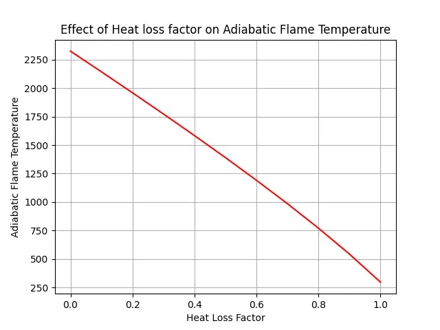
From the above figure it can be observed that with increase in heat loss, the flame temperature decreases as heat is lost from the system.
The flame temperature for heat loss factor of 0.35 for methane is 1678.805K
Case 3. Adiabatic flame temperature variation with respect to Alkane, Alkene, Alkyne (variants of 2 Carbon atoms) :
Constant pressure system and no heat loss is assumed for this case. Adiabatic flame temperature for ethane, ethene and ethyne is computed and compared. The reactions for ethane, ethene and ethyne are as follows :
Ethane

Ethene
 .
.
Ethyne

Python code
"""
stoichometric
C2H6 + 3.5(O2+3.76N2) = 2CO2 + 3H2O + 13.16N2
C2H4 + 3(O2+3.76N2) = 2CO2 + 2H2O + 11.28N2
C2H2 + 2.5(O2+3.76N2) = 2CO2 + H2O + 9.4N2
"""
import cantera as ct
import matplotlib.pyplot as plt
import math
import numpy as np


def h(T, coeffs):
	# Function to evaluate enthalpy

	R = 8.314 #J/mol-K,kJ/kmol-K
	a1 = coeffs[0]
	a2 = coeffs[1]
	a3 = coeffs[2]
	a4 = coeffs[3]
	a5 = coeffs[4]
	a6 = coeffs[5]

	return (a1 + a2*T/2 + a3*pow(T,2)/3 + a4*pow(T,3)/4 + a5*pow(T,4)/5 + a6/T)*R*T

# Low temperatue coefficients

c2h6_coeffs_l = [4.29142492E+00,-5.50154270E-03,5.99438288E-05,-7.08466285E-08,2.68685771E-11,-1.15222055E+04,2.66682316E+00]

c2h4_coeffs_l = [3.95920148E+00,-7.57052247E-03,5.70990292E-05,-6.91588753E-08,2.69884373E-11,5.08977593E+03,4.09733096E+00 ]

c2h2_coeffs_l = [8.08681094E-01,2.33615629E-02,-3.55171815E-05,2.80152437E-08,-8.50072974E-12,2.64289807E+04,1.39397051E+01]

o2_coeffs_l = [3.78245636E+00,-2.99673416E-03,9.84730201E-06,-9.68129509E-09,3.24372837E-12,-1.06394356E+03,3.65767573E+00]

n2_coeffs_l = [0.03298677E+02,0.14082404E-02,-0.03963222E-04,0.05641515E-07,-0.02444854E-10,-0.10208999E+04,0.03950372E+02]

# High temperatue coefficients

n2_coeffs_h = [0.02926640E+02,0.14879768E-02,-0.05684760E-05,0.10097038E-09,-0.06753351E-13,-0.09227977E+04,0.05980528E+02]

co2_coeffs_h = [3.85746029E+00,4.41437026E-03,-2.21481404E-06,5.23490188E-10,-4.72084164E-14,-4.87591660E+04,2.27163806E+00]

h2o_coeffs_h = [3.03399249E+00,2.17691804E-03,-1.64072518E-07,-9.70419870E-11,1.68200992E-14,-3.00042971E+04, 4.96677010E+00]

def f_ethane(T):
# function that represents the root finding problem

	h_co2_p = h(T,co2_coeffs_h)
	h_n2_p = h(T,n2_coeffs_h)
	h_h2o_p = h(T,h2o_coeffs_h)

	H_products = 4*h_co2_p + 26.32*h_n2_p + 6*h_h2o_p

	Tstd = 298.15
	h_c2h6_r = h(Tstd,c2h6_coeffs_l)
	h_o2_r = h(Tstd,o2_coeffs_l)
	h_n2_r = h(Tstd,n2_coeffs_l)

	H_reactants = 2*h_c2h6_r + 7*h_o2_r + 26.32*h_n2_r

	return H_products - H_reactants

def fprime_ethane (T):
	return (f_ethane(T+1e-6) - f_ethane(T))/1e-6

T_guess_ethane = 1500
T_guess_ethene = 1500
T_guess_ethyne = 1500

tol = 1e-4
ct_ethane = 0
ct_ethene = 0
ct_ethyne = 0
alpha = 0.2

while (abs(f_ethane(T_guess_ethane)) > tol):
	T_guess_ethane = T_guess_ethane - alpha*((f_ethane(T_guess_ethane)/fprime_ethane(T_guess_ethane)))
	ct_ethane = ct_ethane + 1

print(T_guess_ethane)

def f_ethene (T):
# function that represents the root finding problem

	h_co2_p = h(T,co2_coeffs_h)
	h_n2_p = h(T,n2_coeffs_h)
	h_h2o_p = h(T,h2o_coeffs_h)

	H_products1 = 2*h_co2_p + 11.28*h_n2_p + 2*h_h2o_p

	Tstd = 298.15
	h_c2h4_r = h(Tstd,c2h4_coeffs_l)
	h_o2_r = h(Tstd,o2_coeffs_l)
	h_n2_r = h(Tstd,n2_coeffs_l)

	H_reactants1 = h_c2h4_r + 3*h_o2_r + 11.28*h_n2_r

	return H_products1 - H_reactants1


def fprime_ethene (T):
	return (f_ethene(T+1e-6) - f_ethene(T))/1e-6

while (abs(f_ethene(T_guess_ethene)) > tol):
	T_guess_ethene = T_guess_ethene - alpha*((f_ethene(T_guess_ethene)/fprime_ethene(T_guess_ethene)))
	ct_ethene = ct_ethene + 1

print(T_guess_ethene)

def f_ethyne (T):
# function that represents the root finding problem

	h_co2_p = h(T,co2_coeffs_h)
	h_n2_p = h(T,n2_coeffs_h)
	h_h2o_p = h(T,h2o_coeffs_h)

	H_products2 = 4*h_co2_p + 18.8*h_n2_p + 2*h_h2o_p

	Tstd = 298.15
	h_c2h2_r = h(Tstd,c2h2_coeffs_l)
	h_o2_r = h(Tstd,o2_coeffs_l)
	h_n2_r = h(Tstd,n2_coeffs_l)

	H_reactants2 = 2*h_c2h2_r + 5*h_o2_r + 18.8*h_n2_r

	return H_products2 - H_reactants2

def fprime_ethyne (T):
	return (f_ethyne(T+1e-6) - f_ethyne(T))/1e-6

while (abs(f_ethyne(T_guess_ethyne)) > tol):
	T_guess_ethyne = T_guess_ethyne - alpha*((f_ethyne(T_guess_ethyne)/fprime_ethyne(T_guess_ethyne)))
	ct_ethyne = ct_ethyne + 1

print(T_guess_ethyne)

T_aft = [T_guess_ethane, T_guess_ethene, T_guess_ethyne]
print (T_aft)

hydrocarbon = ['Ethane (C2H6)','Ethene (C2H4)','Ethyne (C2H2)']
plt.bar(hydrocarbon, T_aft)
plt.xlabel("Type of Hydrocarbon")
plt.ylabel("Adiabatic Flame Temperature")
plt.title("Comparison of AFT between Ethane, Ethene and Ethyne")
plt.show()

#For Ethane

gas = ct.Solution('gri30.xml')
gas.TPX = 298.15,101325,{'C2H6':1, 'O2' :3.5, 'N2' :13.16}

gas.equilibrate('HP','auto')
T_ethane = (gas.T)
print(T_ethane)

#For Ethene

gas = ct.Solution('gri30.xml')
gas.TPX = 298.15,101325,{'C2H4':1, 'O2' :3, 'N2' :11.28}

gas.equilibrate('HP','auto')
T_ethene = (gas.T)
print(T_ethene)

#For Ethyne

gas = ct.Solution('gri30.xml')
gas.TPX = 298.15,101325,{'C2H2':1, 'O2' :2.5, 'N2' :9.4}

gas.equilibrate('HP','auto')
T_ethyne = (gas.T)
print(T_ethyne)

aft = [T_ethane, T_ethene, T_ethyne]

print (aft)

plt.bar(hydrocarbon, aft)
plt.xlabel("Type of Hydrocarbon")
plt.ylabel("Adiabatic Flame Temperature")
plt.title("Comparison of AFT between Ethane, Ethene and Ethyne in Cantera")
plt.show()
Comparison of AFT for ethane, ethene and ethyne in python and cantera
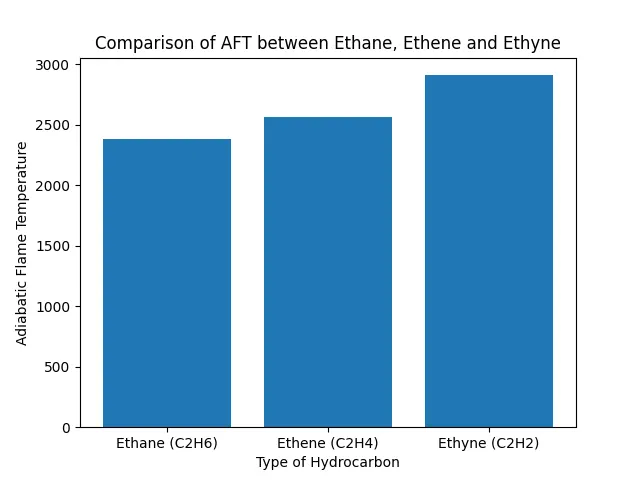
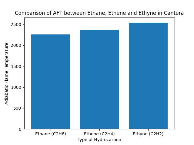
From the above figure, it can be observed AFT for ethane is minimum and AFT for ethyne is maximum. This can be due to presence of higher C-C bonds which requires more energy for combustion. The AFT for ethane is 2379.85K , ethene is 2564.53K , ethyne is 2909.35K in python. The AFT for ethane is 2258.74K , ethene is 2368.64K , ethyne is 2539.67K in cantera.
Case 4. Adiabatic flame temperature variation with respect to a number of Carbon atom chains :
Constant pressure system and no heat loss is assumed for this case. Adiabatic flame temperature for methane, ethane and propane is computed and compared. The reactions for methane, ethane and propane are as follows :
Methane
Ethane
Propane

Python code
"""
program for different values of AFT of methane at different equivalence ratios

stoichometric

CH4 + 2(O2+3.76N2) = CO2 + 2H2O + 7.52N2

C2H6 + 3.5(O2+3.76N2) = 2CO2 + 3H2O + 13.16N2

C3H8 + 5(O2+3.76N2) = 3CO2 + 4H2O + 18.8N2

"""
import cantera as ct
import matplotlib.pyplot as plt
import math
import numpy as np

def h(T, coeffs):
	# Function to evaluate enthalpy

	R = 8.314 #J/mol-K,kJ/kmol-K
	a1 = coeffs[0]
	a2 = coeffs[1]
	a3 = coeffs[2]
	a4 = coeffs[3]
	a5 = coeffs[4]
	a6 = coeffs[5]

	return (a1 + a2*T/2 + a3*pow(T,2)/3 + a4*pow(T,3)/4 + a5*pow(T,4)/5 + a6/T)*R*T

# Low temperatue coefficients

ch4_coeffs_l = [5.14987613E+00,-1.36709788E-02,4.91800599E-05,-4.84743026E-08,1.66693956E-11,-1.02466476E+04,-4.64130376E+00]

c2h6_coeffs_l = [4.29142492E+00,-5.50154270E-03,5.99438288E-05,-7.08466285E-08,2.68685771E-11,-1.15222055E+04,2.66682316E+00]

c3h8_coeffs_l = [0.93355381E+00,0.26424579E-01,0.61059727E-05,-0.21977499E-07,0.95149253E-11,-0.13958520E+05,0.19201691E+02]

o2_coeffs_l = [3.78245636E+00,-2.99673416E-03,9.84730201E-06,-9.68129509E-09,3.24372837E-12,-1.06394356E+03,3.65767573E+00]

n2_coeffs_l = [0.03298677E+02,0.14082404E-02,-0.03963222E-04,0.05641515E-07,-0.02444854E-10,-0.10208999E+04,0.03950372E+02]

# High temperatue coefficients

n2_coeffs_h = [0.02926640E+02,0.14879768E-02,-0.05684760E-05,0.10097038E-09,-0.06753351E-13,-0.09227977E+04,0.05980528E+02]

co2_coeffs_h = [3.85746029E+00,4.41437026E-03,-2.21481404E-06,5.23490188E-10,-4.72084164E-14,-4.87591660E+04,2.27163806E+00]

h2o_coeffs_h = [3.03399249E+00,2.17691804E-03,-1.64072518E-07,-9.70419870E-11,1.68200992E-14,-3.00042971E+04, 4.96677010E+00]

def f_methane(T):
# function that represents the root finding problem

	h_co2_p = h(T,co2_coeffs_h)
	h_n2_p = h(T,n2_coeffs_h)
	h_h2o_p = h(T,h2o_coeffs_h)

	H_products = h_co2_p + 7.52*h_n2_p + 2*h_h2o_p

	Tstd = 298.15
	h_ch4_r = h(Tstd,ch4_coeffs_l)
	h_o2_r = h(Tstd,o2_coeffs_l)
	h_n2_r = h(Tstd,n2_coeffs_l)

	H_reactants = h_ch4_r + 2*h_o2_r + 7.52*h_n2_r

	return H_products - H_reactants

def fprime_methane (T):
	return (f_methane(T+1e-6) - f_methane(T))/1e-6

T_guess_methane = 1500
T_guess_ethane = 1500
T_guess_propane = 1500

tol = 1e-4
ct_methane = 0
ct_ethane = 0
ct_propane = 0
alpha = 0.2

while (abs(f_methane(T_guess_methane)) > tol):
	T_guess_methane = T_guess_methane - alpha*((f_methane(T_guess_methane)/fprime_methane(T_guess_methane)))
	ct_methane = ct_methane + 1

print(T_guess_methane)

def f_ethane (T):
# function that represents the root finding problem

	h_co2_p = h(T,co2_coeffs_h)
	h_n2_p = h(T,n2_coeffs_h)
	h_h2o_p = h(T,h2o_coeffs_h)

	H_products1 = 4*h_co2_p + 26.32*h_n2_p + 6*h_h2o_p

	Tstd = 298.15
	h_c2h6_r = h(Tstd,c2h6_coeffs_l)
	h_o2_r = h(Tstd,o2_coeffs_l)
	h_n2_r = h(Tstd,n2_coeffs_l)

	H_reactants1 = 2*h_c2h6_r + 7*h_o2_r + 26.32*h_n2_r

	return H_products1 - H_reactants1


def fprime_ethane (T):
	return (f_ethane(T+1e-6) - f_ethane(T))/1e-6

while (abs(f_ethane(T_guess_ethane)) > tol):
	T_guess_ethane = T_guess_ethane - alpha*((f_ethane(T_guess_ethane)/fprime_ethane(T_guess_ethane)))
	ct_ethane = ct_ethane + 1

print(T_guess_ethane)

def f_propane (T):
# function that represents the root finding problem

	h_co2_p = h(T,co2_coeffs_h)
	h_n2_p = h(T,n2_coeffs_h)
	h_h2o_p = h(T,h2o_coeffs_h)

	H_products2 = 3*h_co2_p + 18.8*h_n2_p + 4*h_h2o_p

	Tstd = 298.15
	h_c3h8_r = h(Tstd,c3h8_coeffs_l)
	h_o2_r = h(Tstd,o2_coeffs_l)
	h_n2_r = h(Tstd,n2_coeffs_l)

	H_reactants2 = h_c3h8_r + 5*h_o2_r + 18.8*h_n2_r

	return H_products2 - H_reactants2

def fprime_propane (T):
	return (f_propane(T+1e-6) - f_propane(T))/1e-6

while (abs(f_propane(T_guess_propane)) > tol):
	T_guess_propane = T_guess_propane - alpha*((f_propane(T_guess_propane)/fprime_propane(T_guess_propane)))
	ct_propane = ct_propane + 1

print(T_guess_propane)

T_aft = [T_guess_methane, T_guess_ethane, T_guess_propane]
print (T_aft)

hydrocarbon = ['Methane (CH4)','Ethane (C2H6)','Propane (C3H8)']
plt.bar(hydrocarbon, T_aft)
plt.xlabel("Type of Hydrocarbon")
plt.ylabel("Adiabatic Flame Temperature")
plt.title("Comparison of AFT between Methane, Ethane and Propane")
plt.show()

#For Methane

gas = ct.Solution('gri30.xml')
gas.TPX = 298.15,101325,{'CH4':1, 'O2' :2, 'N2' :7.52}

gas.equilibrate('HP','auto')
T_methane = (gas.T)

print(T_methane)

#For Ethane

gas = ct.Solution('gri30.xml')
gas.TPX = 298.15,101325,{'C2H6':1, 'O2' :3.5, 'N2' :13.16}

gas.equilibrate('HP','auto')
T_ethane = (gas.T)

print(T_ethane)

#For Propane

gas = ct.Solution('gri30.xml')
gas.TPX = 298.15,101325,{'C3H8':1, 'O2' :5, 'N2' :18.8}

gas.equilibrate('HP','auto')
T_propane = (gas.T)

print(T_propane)

aft = [T_methane, T_ethane, T_propane]

plt.bar(hydrocarbon, aft)
plt.xlabel("Type of Hydrocarbon")
plt.ylabel("Adiabatic Flame Temperature")
plt.title("Comparison of AFT between Methane, Ethane and Propane in Cantera")
plt.show()
Comparison of AFT for methane, ethane and propane in python and cantera
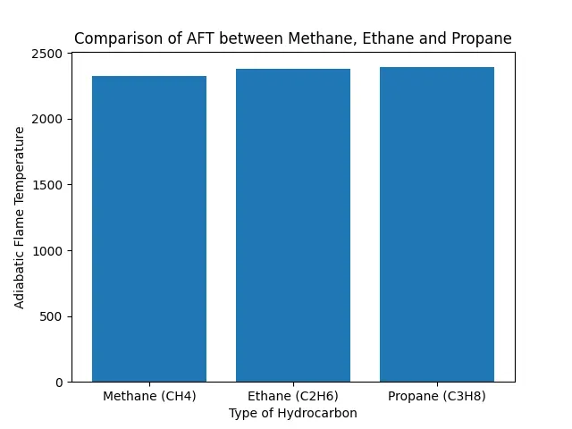
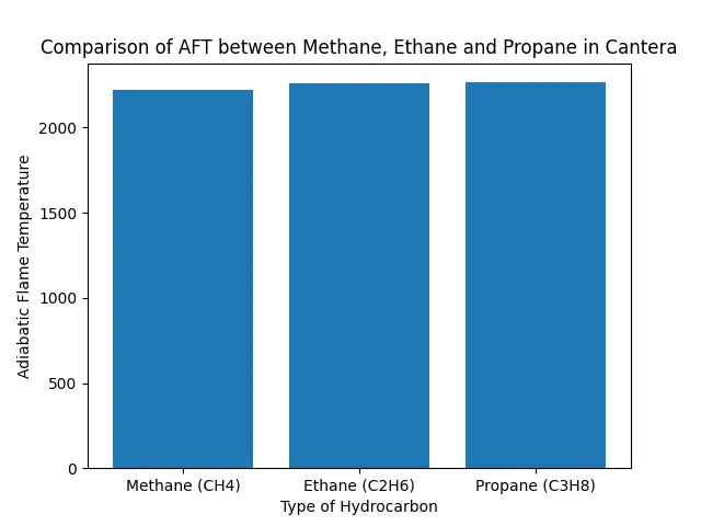
From the above figure, it can be observed AFT for methane is minimum and AFT is maximum for propane. The AFT for methane is 2325.598K , ethane is 2379.85K , propane is 2392.097K in python. The AFT for methane is 2224.62K , ethane is 2258.17K , propane is 2265.701K in cantera.