Week 7 - Simulation of a 1D Super-sonic nozzle flow simulation using Macormack Method
Objective : To simulate the isentropic flow through a quasi 1D subsonic-supersonic nozzle. To derive both the conservation and non-conservation forms of the governing equations and solve them using the Maccormack's technique and to determine the steady-state temperature distribution for the flow-field variables and investigate the difference between the two forms of governing equations by comparing their solutions.
Flow Condition
The flow considered is an isentropic flow through a quasi 1D convergent divergent nozzle. The flow at the inlet of the nozzle comes from a reservoir whose pressure and temperature are p0 and T0. Area of the reservoir is considered to be very large and hence velocity at the inlet of the nozzle is considered to be very small (tends to 0). The velocity is subsonic (M<1) at the convergent part, sonic (M=1) at the throat and supersonic (M>1) at the divergent part of the nozzle. The pressure, velocity, temperature and Mach number at the exit are taken as pe, Te, Ve and Me respectively.
Governing equations
The governing equations can be in conservation and non-conservation forms. The control volume is fixed while deriving the equations for conservation form whereas the control volume is moving while deriving the equations for non conservation form. For a particular flow either of the two forms can be used but each form has its own advantages which makes one form more suitable than other. For this problem, solutions are obtained for both conservation and non-conservation form of governing equations. The governing equations can be in dimensional and non-dimensional form. While dealing with flow related to the nozzles, generally non-dimensional form of governing equations are used.
Non conservation form
The non dimensional governing equations for non conservation form are as follows :
Continuity Equation

Momentum Equation
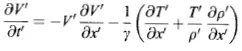
Energy Equation

The above equations are solved using Maccormack's technique and the values of density, velocity and temperature are obtained. Since these values are in non-dimensional form, pressure ratio and Mach number can be obtained as follows :
p = ρT
Mach number = v/√T
Maccormack Method
Maccormack method is an explicit finite difference method and is second order accurate for both space and time derivatives. This method is widely used discretization scheme to obtain numerical solution for hyperbolic PDE's. The results obtained from this method are satisfactory and are close to the actual values. Maccormack's technique uses a two step predictor and corrector sequence. It uses forward difference on predictor and backward difference on corrector.
The Maccormack Method applied on continuity equation is as follows :
Initially in the continuity equation, the space derivatives on RHS are replaced with forward difference.
The predicted density value is given by
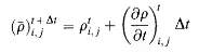
Then in the corrector step, the space derivatives on RHS are replaced with backward difference.
Then the average of predictor and corrector time values are calculated.
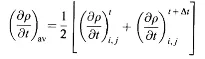
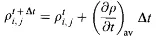
The final value of density at time t+Δt is obtained as
Calculation of time step
The governing equations are hyperbolic with respect to time. The stability criteria for hyperbolic equations is CFL number ≤1
At a given grid point, time step is given by
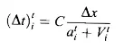
Δt is the time step
C is the CFL number
a is the local speed of sound
V is the flow velocity
Δ𝑥 is the grid size
(Δt) is calculated for all the grid points and then the minimum value is chosen as the timestep

Time step calculation method is same for both non conservation and conservation form.
Initial Conditions
The initial condition of flow field variables are given as function of 𝑥 (distance along the length of nozzle).
The initial condtions for non conservative form at t = 0 are as follows :
ρ = 1 - 0.3146𝑥
T = 1 - 0.2314𝑥
V = (0.1 + 1.09𝑥)T1/2
Nozzle shape
The length of nozzle is 3m. The throat of nozzle is at 1.5m. The nozzle section is convergent for x<1.5m and divergent for x>1.5m. The nozzle shape is specified by A and is held fixed independent of time. The profile of nozzle is a parabolic distribution given by:
A = 1 + 2.2(𝑥 - 1.5)2 for 0≤𝑥≤3
Boundary conditions
At the inlet, one floating variable is used. The boundary condition at inlet is given as
V1 = 2V2 - V3
At the outlet, three floating variables are used. The boundary condition at outlet is given as
VN = 2VN-1 - VN-2
ρN = 2ρN-1 - ρN-2
TN = 2TN-1 - TN-2
Code for non conservation form
clear all
close all
clc

% non conservative form
% inputs
n = 31;
x = linspace (0,3,n);
dx= x(2)-x(1);
gamma = 1.4;
n_throat = (n+1)/2;

% calculate initial profiles
rho = 1-0.3146.*x;
t = 1 - 0.2314.*x;
v = (0.1+1.09*x).*t.^0.5;
CFL = 0.5;
% area
a = 1+2.2*(x-1.5).^2;

% Time steps
% using courant number criteria
nt = 1400;
dt = min(CFL.*dx./(sqrt(t)+v));

% Outer time loop
for k = 1:nt

    rho_old = rho;
    v_old = v;
    t_old = t;

    % Predictor method

    for j = 2:n-1
        % drho_dt_p = -rho(j)*(v(j+1)-v(j))/dx-rho(j)*v(j)*(log(a(j+1)-log(a(j))))/dx - v(j)*(rho(j+1)-rho(j))/dx;
        dvdx = (v(j+1)-v(j))/dx;
        drhodx = (rho(j+1)-rho(j))/dx;
        % t is the temperature
        dtdx = (t(j+1)-t(j))/dx;
        dlogadx = (log(a(j+1))-log(a(j)))/dx;

        % continuity equation
        drhodt_p(j) = -rho(j)*dvdx - rho(j)*v(j)*dlogadx - v(j)*drhodx;

        % momentum equation
        dvdt_p(j) = -v(j)*dvdx - (1/gamma)*(dtdx + (t(j)/rho(j)*drhodx));

        % energy equation
        dtdt_p(j) = -v(j)*dtdx - (gamma-1)*t(j)*(dvdx + v(j)*dlogadx);

        % solution update
        rho(j) = rho(j) + drhodt_p(j)*dt;
        v(j) = v(j)+ dvdt_p(j)*dt;
        t(j) = t(j)+ dtdt_p(j)*dt;
    end

    % corrector method
for j = 2:n-1
        % drho_dt_p = -rho(j)*(v(j+1)-v(j))/dx-rho(j)*v(j)*(log(a(j+1)-log(a(j))))/dx - v(j)*(rho(j+1)-rho(j))/dx;
        dvdx = (v(j)-v(j-1))/dx;
        drhodx = (rho(j)-rho(j-1))/dx;
        % t is the temperature
        dtdx = (t(j)-t(j-1))/dx;
        dlogadx = (log(a(j))-log(a(j-1)))/dx;

        % continuity equation
        drhodt_c(j) = -rho(j)*dvdx - rho(j)*v(j)*dlogadx - v(j)*drhodx;

        % momentum equation
        dvdt_c(j) = -v(j)*dvdx - (1/gamma)*(dtdx + (t(j)/rho(j)*drhodx));

        % energy equation
        dtdt_c(j) = -v(j)*dtdx - (gamma-1)*t(j)*(dvdx + v(j)*dlogadx);

end
    % Compute the average time derivative
    drhodt = 0.5*(drhodt_p + drhodt_c);
    dvdt = 0.5*(dvdt_p +dvdt_c);
    dtdt = 0.5*(dtdt_p + dtdt_c);

    % final solution update
    for i = 2:n-1
    rho(i) = rho_old(i) + drhodt(i)*dt;
    v(i) = v_old(i) + dvdt(i)*dt;
    t(i) = t_old(i) + dtdt(i)*dt;
    end

     M = v./t.^0.5;
     p = rho.*t;
     m = rho.*a.*v;

     M_throat(k) = M(n_throat);
     p_throat(k) = p(n_throat);
     t_throat(k) = t(n_throat);
     rho_throat(k) = rho(n_throat);

    % Apply the boundary conditions
    % inlet boundary condition
    v(1) = 2*v(2) - v(3);

    % outlet
    rho(n) = 2*rho(n-1) - rho(n-2);
    v(n) = 2*v(n-1) - v(n-2);
    t(n) = 2*t(n-1) - t(n-2);

     if (k==1)
        plot(x,m,'y','linewidth',1.5)
    else if (k==50)
            plot (x,m,'r','linewidth',1.5)
        else if (k==100)
                 plot (x,m,'m','linewidth',1.5)
                         else if (k==200)
                                 plot (x,m,'b','linewidth',1.5)
                                 else if (k==700)
                                         plot (x,m,'k','linewidth',1.5)
                                     end
                             end
                     end
        end
    end
 hold on


end
grid on
axis ([0 3 0 2.5])
legend('1 time step','50 time steps','100 time steps','200 time steps','700 time steps')
xlabel('Nozzle distance (x/L)')
ylabel('Non dimensional mass flow rate')
title ('Mass flow rate along nozzle length at different time steps')

figure(2)
subplot(4,1,1)
plot(x,M,'r','linewidth',1.5)
ylabel('Mach Number')
title ('Variation of variables along nozzle length')
subplot(4,1,2)
plot(x,p,'linewidth',1.5)
ylabel('Pressure')
subplot(4,1,3)
plot(x,rho,'g','linewidth',1.5)
ylabel('Density')
subplot(4,1,4)
plot(x,t,'m','linewidth',1.5)
xlabel('Nozzle distance (x/L)')
ylabel('Temperature')

figure(3)
subplot(4,1,1)
plot(rho_throat,'r','linewidth',1.5)
ylabel('Density')
title ('Variation of variables with time')
subplot(4,1,2)
plot(t_throat,'linewidth',1.5)
ylabel('Temperature')
subplot(4,1,3)
plot(p_throat,'g','linewidth',1.5)
ylabel('Pressure')
subplot(4,1,4)
plot(M_throat,'m','linewidth',1.5)
xlabel('Number of time Steps')
ylabel('Mach Number')
Conservation form
The non dimensional governing equations for conservation form are as follows
Continuity Equation

Momentum Equation

Energy Equation

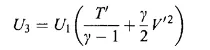
Due to the difficulty of solving the above equations, the above equations are expressed in the form of solution vector U, flux vector F and source term J


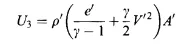
U1, U2 and U3 forms solution vector

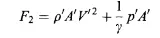

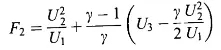
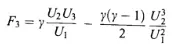
F1, F2 and F3 forms flux vector

J2 is the source term
Substituting U1, U2, U3, F1, F2, F3 and J2 in Continuity, momentum and energy equations, the new equations are as follows :
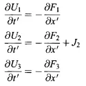
For ease of solving the problem F1, F2 and F3 are written in the form of U1, U2 and U3

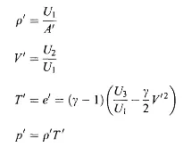
U1, U2 and U3 obtained by solving the above equations need to be converted back in the form of primitive variables which are as follows :
Initial Conditions
For conservative form, initial conditions are given by,



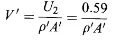
Initial mass flow rate is assumed to be a constant value 0.579 from which initial velocity is calculated as
The area profile for conservative form is same as the non-conservative form
Boundary conditions
At inlet, boundary condition is given by


V(1) = U2(1)/U1(1)
At outlet, boundary condition is given by
(U1)N = 2(U1)N-1 - (U1)N-2
(U2)N = 2(U2)N-1 - (U2)N-2
(U3)N = 2(U3)N-1 - (U3)N-2
Code for conservation form
clear all
close all
clc

% inputs
n = 31;
x = linspace (0,3,n);
dx= x(2)-x(1);
gamma = 1.4;
n_throat = (n+1)/2;

% calculate initial profiles
for i=1:n
if x(i)<=0.5
rho(i) = 1;
t(i) = 1;
end

if x(i)>0.5 && x(i)<=1.5
rho(i) = 1-0.366*(x(i)-0.5);
t(i) =  1-0.167*(x(i)-0.5);
end

if x(i)>1.5
rho(i) = 0.634-0.3879*(x(i)-1.5);
t(i) =  0.833-0.3507*(x(i)-1.5);
end

end
% area
a = 1+2.2*(x-1.5).^2;

u1 = rho.*a;
v = 0.59./(u1);
u2 = rho.*a.*v;
u3 = u1.*(t./(gamma-1)+ gamma*0.5*v.^2);

nt = 1400;
CFL = 0.5;
dt = min(CFL*(dx./(sqrt(t)+v)));

for k=1:nt

    u1_old = u1;
    u2_old = u2;
    u3_old = u3;

    f1 = u2;
    f2 = u2.^2./u1 + (gamma-1)/gamma.*(u3-0.5.*gamma.*u2.^2./u1);
    f3 = (gamma.*u2.*u3./u1)-(0.5.*gamma.*(gamma-1)*u2.^3./u1.^2);


    for i=2:n-1
        dadx = (a(i+1)-a(i))/dx;
        j2(i) = (1/gamma)*rho(i)*t(i)*dadx;
        du1dt_p(i) = -(f1(i+1)-f1(i))/(dx);
        du2dt_p(i) = -(f2(i+1)-f2(i))/(dx)+j2(i);
        du3dt_p(i) = -(f3(i+1)-f3(i))/(dx);

        u1(i) = u1(i) +  du1dt_p(i)*dt;
        u2(i) = u2(i) +  du2dt_p(i)*dt;
        u3(i) = u3(i) +  du3dt_p(i)*dt;
    end

    rho = u1./a;
    t = (gamma-1)*((u3./u1)- gamma*0.5*(u2./u1).^2);
    v = u2./u1;

    f1new = u2;
    f2new = u2.^2./u1 + (gamma-1)/gamma.*(u3-0.5.*gamma.*u2.^2./u1);
    f3new = (gamma.*u2.*u3./u1)-(0.5.*gamma.*(gamma-1)*u2.^3./u1.^2);

    for j=2:n-1
        dadx = (a(j)-a(j-1))/dx;
        j2(j) = (1/gamma)*rho(j)*t(j)*dadx;

        du1dt_c(j) = -(f1new(j)-f1new(j-1))/dx;
        du2dt_c(j) = -(f2new(j)-f2new(j-1))/(dx)+j2(j);
        du3dt_c(j) = -(f3new(j)-f3new(j-1))/(dx);
    end

    du1dt = 0.5*(du1dt_p+du1dt_c);
    du2dt = 0.5*(du2dt_p+du2dt_c);
    du3dt = 0.5*(du3dt_p+du3dt_c);

    %Final solution update
    for q = 2:n-1
        u1(q) = u1_old(q)+ du1dt(q)*dt;
        u2(q) = u2_old(q)+ du2dt(q)*dt;
        u3(q) = u3_old(q)+ du3dt(q)*dt;

    end

    %Boundary condition
     %inlet
     u1(1) = a(1);
     u2(1) = 2*u2(2)-u2(3);
     v(1) = u2(1)/u1(1);
     u3(1) = u1(1)*(t(1)/(gamma-1)+ gamma*0.5*v(1)^2);

     %outlet
     u1(n) = 2*u1(n-1)-u1(n-2);
     u2(n) = 2*u2(n-1)-u2(n-2);
     u3(n) = 2*u3(n-1)-u3(n-2);

     % final primitive variables
     rho = u1./a;
     t = (gamma-1)*((u3./u1)- gamma*0.5*(u2./u1).^2);
     v = u2./u1;
     p = rho.*t;
     M = v./(t.^0.5);
     m = u2;

     M_throat(k) = M(n_throat);
     p_throat(k) = p(n_throat);
     t_throat(k) = t(n_throat);
     rho_throat(k) = rho(n_throat);

     figure(1)
     if (k==1)
         plot(x,m,'r','linewidth',1.5)
         else if (k==50)
                 plot (x,m,'g','linewidth',1.5)
                  else if (k==100)
                           plot (x,m,'m','linewidth',1.5)
                           else if (k==200)
                                   plot (x,m,'b','linewidth',1.5)
                                   else if (k==700)
                                            plot (x,m,'k','linewidth',1.5)
                                       end
                               end
                      end
             end
     end

hold on

end
grid on
legend('1 time step','50 time steps','100 time steps','200 time steps','700 time steps')
xlabel('Nozzle distance (x/L)')
ylabel('Non dimensional mass flow rate')
title ('Mass flow rate along nozzle length at different time steps')

figure(2)
subplot(4,1,1)
plot(x,M,'r','linewidth',1.5)
ylabel('Mach Number')
title ('Variation of variables along nozzle length')
subplot(4,1,2)
plot(x,p,'linewidth',1.5)
ylabel('Pressure')
subplot(4,1,3)
plot(x,rho,'g','linewidth',1.5)
ylabel('Density')
subplot(4,1,4)
plot(x,t,'m','linewidth',1.5)
xlabel('Non Dimensional nozzle length (x/L)')
ylabel('Temperature')

figure(3)
axis ([0 3 0 1])
subplot(4,1,1)
plot(rho_throat,'r','linewidth',1.5)
ylabel('Density')
title ('Variation of variables with time')
subplot(4,1,2)
plot(t_throat,'linewidth',1.5)
ylabel('Temperature')
subplot(4,1,3)
plot(p_throat,'g','linewidth',1.5)
ylabel('Pressure')
subplot(4,1,4)
plot(M_throat,'m','linewidth',1.5)
xlabel('Number of Time Steps')
ylabel('Mach Number')

figure(4)
m1 = [0.5877,0.5936,0.5890,0.5910,0.5892,0.5894,0.5884,0.5880,0.5872,0.5865,0.5858,0.5852,0.5847,0.5842,0.5839,0.5837,0.5837,0.5840,0.5847,0.5856,0.5866,0.5876,0.5886,0.5895,0.5903,0.5911,0.5915,0.5925,0.5917,0.5955,0.5856];
% values copied from non conservative program to compare mass flow rate
m2 = 0.579*ones(1,31);
plot (x,m1,'b','linewidth',1.5)
hold on
plot (x,m,'k','linewidth',1.5)
hold on
plot (x,m2,'--r','linewidth',1.5)
grid on
legend ('non - conservative','conservative','exact solution')
xlabel ('Non Dimensional nozzle length (x/L)')
ylabel ('Non Dimensional mass flow rate')
title ('Comparison of mass flow rates')
Results
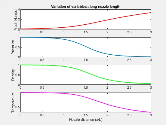
Steady state distribution of primitive variables inside the nozzle
Non-conservation form
Conservation form
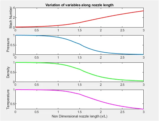
The above graph shows the steady state profile of primitive variables for both non conservation and conservation form. The profile for all flow variables in both forms matches very closely with the analytical solution. The parameters considered are Mach number, pressure, density and temperature. Along the length of the nozzle especially after throat section, the velocity is increasing whereas pressure, density and temperature are decreasing.
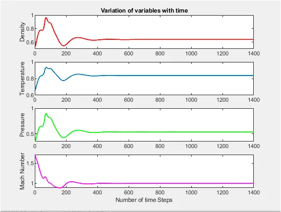
Timewise variation of primitive variables
Non conservation form
Conservation form
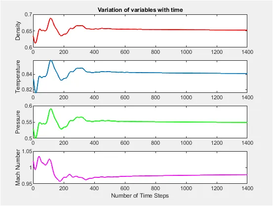
In the initial time steps for both non conservation and conservation forms, time derivatives are large with lot of fluctuations. Hence, the changes in values from one time step to next time step is more for initial time steps. As the number of time step increases, the changes in values between time steps becomes smaller. After certain number of timesteps, the solution reaches steady state. The plots in the graph are similar to the plots given in the reference book (Anderson). At steady state, the residuals of non conservation form is smaller than conservation form
Mass flow rate distribution at different time steps inside the nozzle for non conservation form
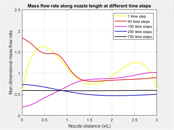
The mass flow rate profile at first time step is like sine wave. The variaton of mass flow rate along the length of the nozzle is large for initial few time steps. This is due to unsteady compression and expansion waves through nozzle during transient process. The profile starts to settle down after 200 time steps. From this point, the change in mass flow rate values with increase in time step becomes smaller and the amount of fluctuation also decreases. After 700 time steps, the changes in mass flow rate is negligible and hence the profile becomes straight line. This indicates that the mass flow rate has attained a constant, steady state value throughout the nozzle. At this point, the solution obtained is very close to the exact solution.
Mass flow rate distribution at different time steps inside the nozzle for conservation form
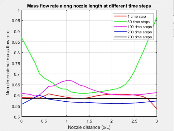
The fluctuations for initial time steps in conservation form is lesser than non conservation form. At 100 time steps, the mass flow rate profile shows humped distribution. After 200 time steps, the profile becomes more stable with less variations. After 700 time steps like non conservation form, the profile becomes a horizontal straight line indicating the solution has reached steady state.
Comparison of normalized flow rates for both forms
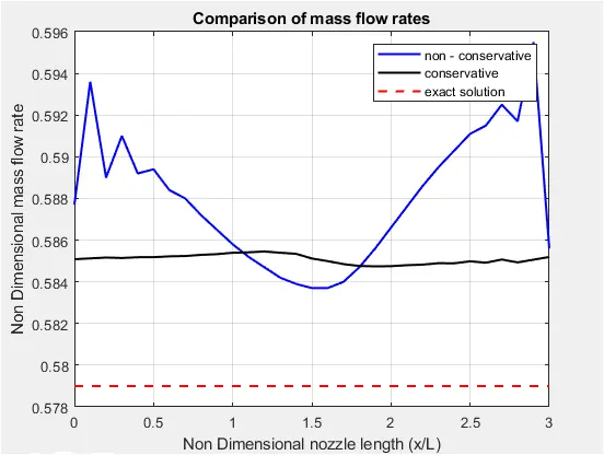
1) In total, the mass flow rate distribution given by conservation form is more closer to constant. The variations given by non conservation form is more than conservation form due to more oscillations at inflow and outflow boundaries.
2) The steady state mass flow rate obtained by conservation form is more closer to the analytical value of 0.579.
3) The conservation form conserves the mass throughout the flow field better as mass flow rate itself is one of the variables in the equations. In non conservation form, the equations are solved for primitive variables. Hence mass flow rate is obtained as a secondary result.
Grid independence test
Grid independence test is done to test the accuracy of solution by changing the grid size. For this purpose, the solutions obtained at (n=31) and (n=61) are tested. Although by increasing the grid points, the steady state results are more closer to the exact analytical solution but the changes in values of primitive variables by increasing the number of grid points is negligible. Hence the solution is grid independent at 31 grid points.
| Solution at throat | Density ratio | Temperature ratio | Pressure ratio | Mach Number |
| Exact analytical solution | 0.634 | 0.833 | 0.528 | 1.000 |
| Non conservation form, numerical solution(31 points) | 0.638 | 0.836 | 0.534 | 0.999 |
| Non conservation form, numerical solution(61 points) | 0.637 | 0.835 | 0.532 | 0.999 |
| Conservation form, numerical solution(31 points) | 0.652 | 0.841 | 0.548 | 0.978 |
| Conservation form, numerical solution(61 points) | 0.639 | 0.835 | 0.533 | 0.997 |