Week 5.1 - Mid term project - Solving the steady and unsteady 2D heat conduction problem

Objective : To solve the 2D heat conduction equation for steady state analysis & transient state snalysis by using the point iterative techniques .The Boundary conditions for the problem are as follows : Top Boundary = 600 K, Bottom Boundary = 900 K, Left Boundary = 400 K, Right Boundary = 800 K. For solving implicit equations methods like Jacobi, Gauss-seidel and Successive over-relaxation are used with absolute error criteria as 1e-4.

Procedure :

Steady State

The 2D steady state heat conduction equation with no heat generation is given by :

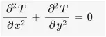
By using second order central difference approximation for the above equation,

The 2d steady state equation becomes

where Tp is the point at which temperature is to be calculated and k is given by

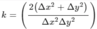
Using this formula, temperature at various points in the domain are calculated

Program :

Initially all the input conditions known for the problem are defined. Then the problem is solved for different iterative methods like Jacobi, Gauss Seidel and SOR. For all the methods, a space loop is defined for x and y directions which is inside the convergence loop with the given condition (error > tolerance). The program is run till the error value falls below the tolerance value. In this way, the number of iterations required to reach the steady state for all the methods are determined.

For unsteady state by implicit method, the temperature values at previous time step are updated in time loop to calculate temperature for new time step;

Code for steady state

clear all
close all
clc

% for steady state
% d2t/dx2+d2t/dy2 = 0;
Tt = 600;
Tb = 900;
Tl = 400;
Tr = 800;

% Tp = (Δx2.Δy2)/(Δx2+Δy2)*((Tr+Tl/Δx2)+Tt+T
Lx = 1;
Ly = 1;
nx = 21;
ny = 21;
x = linspace (0,Lx,nx);
% dx = L/(n-1)
y = linspace (0,Ly,ny);
dx = x(2)-x(1);
dy = y(2)-y(1);

K = 1/(2*(dx^2+dy^2)/(dx^2*dy^2));

T = 600*ones(nx,ny);

T(1,1) = (Tt+Tl)/2;
T(end,end) = (Tb+Tr)/2;
T(end,1) = (Tb+Tl)/2;
T(1,end)= (Tt+Tr)/2;
T(1,2:end-1)= Tt;
T(end,2:end-1) = Tb;
T(2:end-1,1) = Tl;
T(2:end-1,end) = Tr;
Told = T;

iterative_solver = 3;
error = 1;
tolerance = 1e-4;

jacobi_iter = 1;

if iterative_solver ==1
   while (error > tolerance)
       for i = 2:nx-1;
           for j = 2:ny-1;
               T(i,j) = (Told(i-1,j)+Told(i+1,j))*K/dx^2+(Told(i,j-1)+Told(i,j+1))*K/dy^2;
           end
       end
       error = max(max(abs(Told-T)));
       Told = T;
       jacobi_iter = jacobi_iter + 1;
   end
   [C,h] = contourf(x,y,T);
   clabel(C,h)
   colorbar
   colormap(jet)
   set(gca,'YDIR','reverse')
   xlabel('Length in x direction')
   ylabel('Length in y direction')
   title_text = (sprintf('Jacobi iteration number = %d', jacobi_iter));
   title('Steady State Temperature Profile (Jacobian)',title_text);
end


% gs_iter
gs_iter = 1;
if iterative_solver ==2
   while (error > tolerance)
       for i = 2:nx-1;
           for j = 2:ny-1;
               T(i,j) = (T(i-1,j)+T(i+1,j))*K/dx^2+(T(i,j-1)+T(i,j+1))*K/dy^2;
           end
       end
       error = max(max(abs(Told-T)));
       Told = T;
       gs_iter = gs_iter + 1;
   end
   [C,h] = contourf(x,y,T);
   clabel(C,h)
   colorbar
   colormap(jet)
   set(gca,'YDIR','reverse')
   xlabel('Length in x direction')
   ylabel('Length in y direction')
   title_text = (sprintf('Gauss Seidel iteration number = %d', gs_iter));
   title('Steady State Temperature Profile (Gauss Seidel)',title_text);
end

 
% SOR iteration
w = 1.2;
SOR_iter = 1;
if iterative_solver ==3
   while (error > tolerance)
       for i = 2:nx-1;
           for j = 2:ny-1;
               T(i,j) = (1-w)*Told(i,j)+w*((T(i-1,j)+T(i+1,j))*K/dx^2+(T(i,j-1)+T(i,j+1))*K/dy^2);          
           end
       end
       error = max(max(abs(Told-T)));
       Told = T;
       SOR_iter = SOR_iter + 1;
   end
   [C,h] = contourf(x,y,T);
   clabel(C,h)
   colorbar
   colormap(jet)
   set(gca,'YDIR','reverse')
   xlabel('Length in x direction')
   ylabel('Length in y direction')
   title_text = (sprintf('SOR iteration number = %d', SOR_iter));
   title('Steady State Temperature Profile (SOR)',title_text);
end

Results :

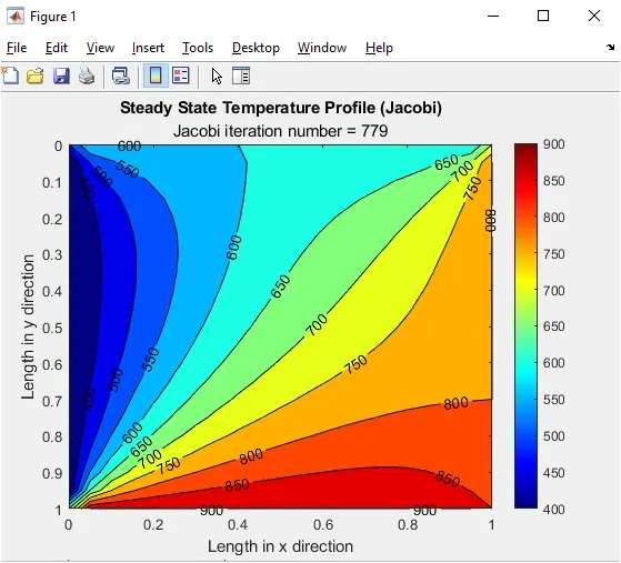
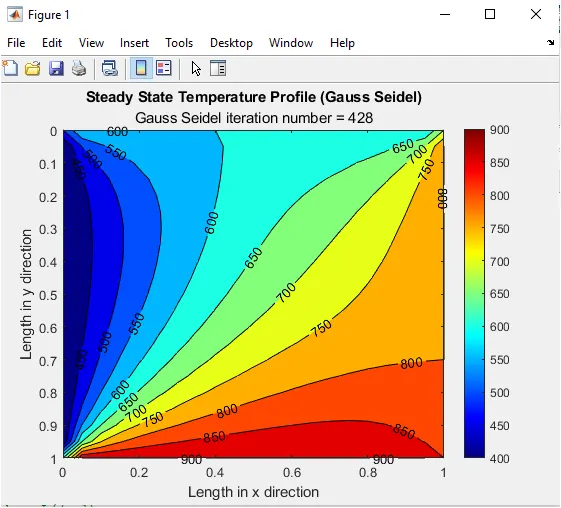
The graphs obtained for 2D steady state heat conduction using Jacobi, Gauss seidel and SOR iterative maethods are as follows:

For Jacobi method,

For Gauss Seidel method,

For SOR method,

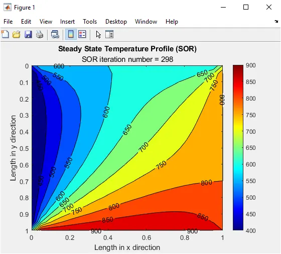
From the above graphs, it can be seen that the number of iterations required to reach steady state are different for different iterative methods. The number of iterations required for Jacobi method is highest followed by Gauss Seidel method. The number of iterations required are least for SOR method. For Jacobi method, the old temperature values are used to compute values for next iteration, hence more number of iterations are required to achieve convergence. For Gauss Seidel method, the new calculated temperature values are used to compute values for next iteration. Since the calculated new values are used for next iteration, the number of iterations required for Gauss Seidel method is less than Jacobi method.SOR (Successive over-relaxation) is a variant of Gauss Seidel method which uses a relaxation factor 'w' to achieve faster convergence. Hence the number of iterations required are least for SOR method.

Unteady State heat conduction

The 2D steady state heat conduction equation without heat generation is given by :

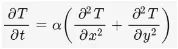
By using second order central difference approximation for the above equation,

For explicit method, the unsteady state heat conduction equation becomes,

where Tp on LHS is the point at which temperature is to be calculated at time step n+1.Tr, Tl, Tt and Tb and Tp on RHS are calculated at time step n

For implicit method, the unsteady state heat conduction equation becomes,

where Tp is the point at which temperature is to be calculated at time step n+1.

k1 = αΔt/Δx² and k2 = αΔt/Δy², where

α is the diffusion coefficient

Tr, Tl, Tt and Tb are calculated at time step n+1

Program

Code for unsteady state by explicit method,

clear all
close all
clc

% for steady state
% d2t/dx2+d2t/dy2 = 0;
Tt = 600;
Tb = 900;
Tl = 400;
Tr = 800;

% Tp = (Δx2.Δy2)/(Δx2+Δy2)*((Tr+Tl/Δx2)+Tt+T
Lx = 1;
Ly = 1;
nx = 21;
ny = 21;
x = linspace (0,Lx,nx);
% dx = L/(n-1)
y = linspace (0,Ly,ny);
dx = x(2)-x(1);
dy = y(2)-y(1);

T = 300*ones(nx,ny);

T(1,1) = (Tt+Tl)/2;
T(end,end) = (Tb+Tr)/2;
T(end,1) = (Tb+Tl)/2;
T(1,end)= (Tt+Tr)/2;
T(1,2:end-1)= Tt;
T(end,2:end-1) = Tb;
T(2:end-1,1) = Tl;
T(2:end-1,end) = Tr;
Told = T;

alpha = 1.4;
t = 0.15;
dt = 0.0001;
CFL = alpha*dt*(1/dx^2+1/dy^2);

K1 = alpha*dt/dx^2;
K2 = alpha*dt/dy^2;
iteration = 1;
nt = t/dt;

for k = 1:nt         % 1500 time steps
    for i = 2:nx-1
        for j = 2:ny-1
            T(i,j) = Told(i,j)+(Told(i-1,j)-2*Told(i,j)+Told(i+1,j))*K1+(Told(i,j-1)-2*Told(i,j)+Told(i,j+1))*K2;
        end
    end
    Told = T;
    iteration = iteration + 1;
end 
[C,h]=contourf(x,y,T);
clabel(C,h)
colorbar
colormap(jet)
set(gca,'YDIR','reverse')
xlabel('Length in x direction')
ylabel('Length in y direction')
title_text = (sprintf('Number of iterations =%d', iteration'));
title ('Unsteady Temperature Profile (explicit)',title_text)

Code for unsteady state by implicit method

clear all
close all
clc

% for steady state
% d2t/dx2+d2t/dy2 = 0;
Tt = 600;
Tb = 900;
Tl = 400;
Tr = 800;

Lx = 1;
Ly = 1;
nx = 21;
ny = 21;
x = linspace (0,Lx,nx);
% dx = L/(n-1)
y = linspace (0,Ly,ny);
dx = x(2)-x(1);
dy = y(2)-y(1);

T = 600*ones(nx,ny);

T(1,1) = (Tt+Tl)/2;
T(end,end) = (Tb+Tr)/2;
T(end,1) = (Tb+Tl)/2;
T(1,end)= (Tt+Tr)/2;
T(1,2:end-1)= Tt;
T(end,2:end-1) = Tb;
T(2:end-1,1) = Tl;
T(2:end-1,end) = Tr;

Told = T;
Tprevious = T;

alpha = 1.4;
dt = 0.0001;
t = 0.15;
nt = t/dt; % 1500 time steps

K1 = alpha*dt/dx^2;
K2 = alpha*dt/dy^2;
CFL = K1+K2
p = 1/(1+2*K1+2*K2);

iterative_solver = 3;
tolerance = 1e-4;

% jacobi iteration
jacobi_iter = 1;

if iterative_solver ==1
    for k = 1:nt % time loop (1500 time steps)
        error = 100;
        while (error > tolerance)% convergence loop
            for i = 2:nx-1 % space loop
                for j = 2:ny-1
                    T(i,j) = (p*Tprevious(i,j))+(Told(i-1,j)+Told(i+1,j))*K1*p+(Told(i,j-1)+Told(i,j+1))*K2*p;
                end
            end
            error = max(max(abs(Told-T)));
            Told = T;
            jacobi_iter = jacobi_iter + 1; 
        end   
        Tprevious = T;
    end
    [C,h]=contourf(x,y,T);
    clabel(C,h)
    colorbar
    colormap(jet)
    set(gca,'YDIR','reverse')
    xlabel('Length in x direction')
    ylabel('Length in y direction')
    title_text = (sprintf('Jacobi iteration number = %d', jacobi_iter));
    title('Unsteady State Temperature Profile (Jacobi)',title_text)
end

% Gauss Seidel iteration
gs_iter = 1;
if iterative_solver ==2
    for k = 1:1500 % time loop
        error = 100;
        while (error > tolerance)% convergence loop
            for i = 2:nx-1 % space loop
                for j = 2:ny-1
                    T(i,j) = (p*Tprevious(i,j))+(T(i-1,j)+T(i+1,j))*K1*p+(T(i,j-1)+T(i,j+1))*K2*p;
                end
            end
            error = max(max(abs(Told-T)));
            Told = T;
            gs_iter = gs_iter + 1; 
            Tprevious = T;
        end 
    end
    [C,h]=contourf(x,y,T);
    clabel(C,h)
    colorbar
    colormap(jet)
    set(gca,'YDIR','reverse')
    xlabel('Length in x direction')
    ylabel('Length in y direction')
    title_text = (sprintf('Gauss Seidel iteration number = %d', gs_iter));
    title('Unsteady State Temperature Profile (Gauss Seidel)',title_text)
end

% SOR iteration
SOR_iter = 1;
w = 1.2;
if iterative_solver ==3
    for k = 1:1500 % time loop
        error = 100;
        while (error > tolerance)% convergence loop
            for i = 2:nx-1 % space loop
                for j = 2:ny-1
                    T(i,j) = (1-w)*Told(i,j)+w*((p*Tprevious(i,j))+(T(i-1,j)+T(i+1,j))*K1*p+(T(i,j-1)+T(i,j+1))*K2*p);
                end
            end
            error = max(max(abs(Told-T)));
            Told = T;
            SOR_iter = SOR_iter + 1; 
            Tprevious = T;
        end    
    end
    [C,h]=contourf(x,y,T);
    clabel(C,h)
    colorbar
    colormap(jet)
    set(gca,'YDIR','reverse')
    xlabel('Length in x direction')
    ylabel('Length in y direction')
    title_text = (sprintf('SOR iteration number = %d', SOR_iter));
    title('Unsteady State Temperature Profile (SOR)',title_text)
end
    
    
                

Results

Temperature profile of unsteady state heat conduction by explicit method

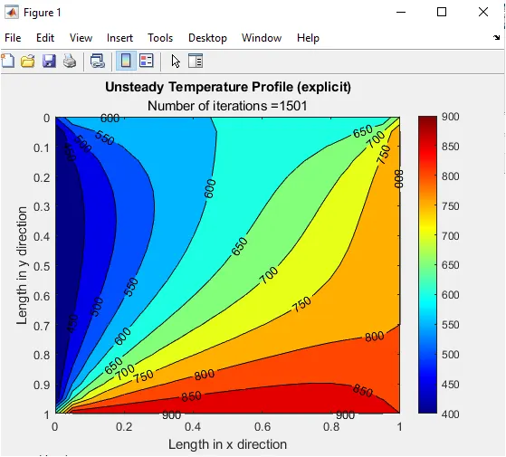
Iterative methods are not required for solving unsteady state heat conduction equation by explicit method. Temperature at top, bottom, left and right node points are calculated at time step n which are known. Hence there is only one unknown in the whole equation for which convergence criteria is not required.

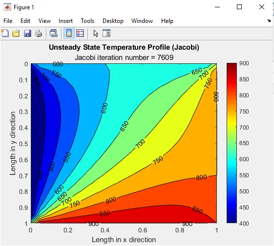
Temperature profile of unsteady state heat conduction for explicit method by Jacobi iterative method

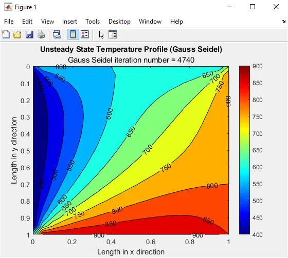
The temperature profile of unsteady state heat conduction by explicit method by Gaus Seidel iterative method

The temperature profile of unsteady state heat conduction by explicit method by SOR method

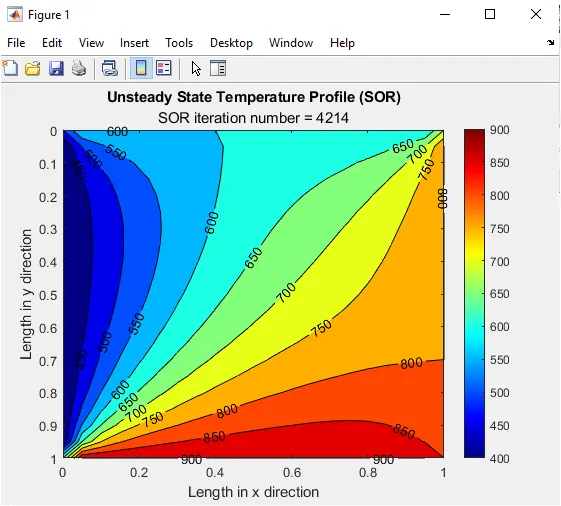
From the above graphs, it can be seen that the number of iterations required to reach steady state are different for different iterative methods.

The number of iterations required for temperature calculation of unsteady heat conduction by explicit method is more than the iterations required for steady state heat conduction.

In case of transient solution, explicit method requires lesser number of iterations and are easier to solve than implicit methods. This is because in case of explicit method, the temperatures at left, right, top and bottom nodes are calculated at time step n which are known whereas in case of implicit method, the temperatures at left, right, top and bottom nodes are calculated at time step n+1 which are not known. Hence more number of iterations are needed for implicit methods to achieve convergence.

For implicit methods also, the number of iterations required for Jacobi method is highest followed by Gauss Seidel method. The number of iterations required are least for SOR method.