Week 9 - Parametric study on Gate valve.

Objective

To perform a parametric study on the gate valve simulation by setting the opening from 10 % to 80%.

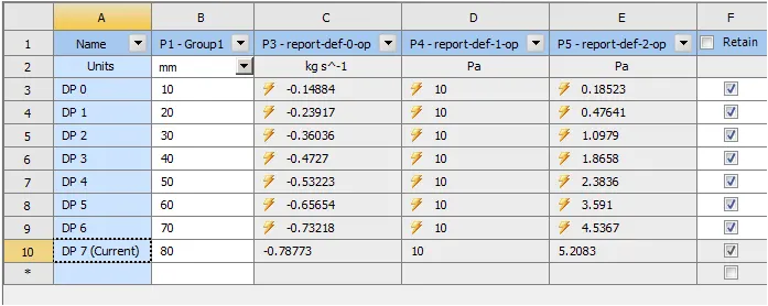
• Obtain the mass flow rates at the outlet for each design point.
• Calculate the flow coefficient and flow factor for each opening and plot the graph.
• Discuss the results of the mass flow rate and flow coefficient.

Introduction

A gate valve controls the media's flow by lifting the gate (open) and lowering the gate (closed). A gate valve's distinct feature is the straight-through unobstructed passageway, which induces minimal pressure loss over the valve. Gate valves are available in many options, including various sizes, materials, temperature and pressure ratings, and gate and bonnet designs.

A gate valve's main components are body, seat, gate, stem, bonnet, and actuator as shown in the figure. The primary operation mechanism is straightforward. Turning the handwheel rotates the stem, which moves the gate up or down via the threads. Lifting the gate from the path of the flow, the valve opens. Lowering the gate to its closed position seals the bore resulting in a full closure of the valve.

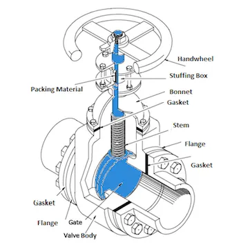
Gate valve geometry

Importing the CAD model of gate valve into spaceclaim.

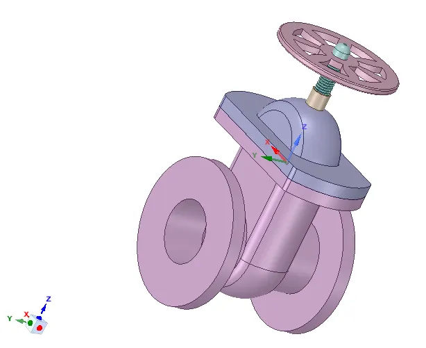
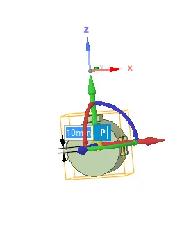
After importing the geometry, hide the other parts so we can clearly see the gate disc. Then select the gate disc and move it in upward direction by 10mm. While giving 10mm lift, select the P icon so that we can parameterize the lift movement.

We need fluid volume for analysis, so we go to prepare-Volume extract in order to get the fluid volume.

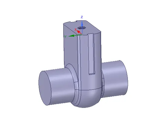
After setting the lift of gate disc, pull both the faces at inlet and outlet of bottom section by 800mm.

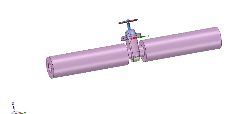
For analysis, we have to make sure to get the desired fluid flow region so we update volume body in context to get the region of fluid flow.

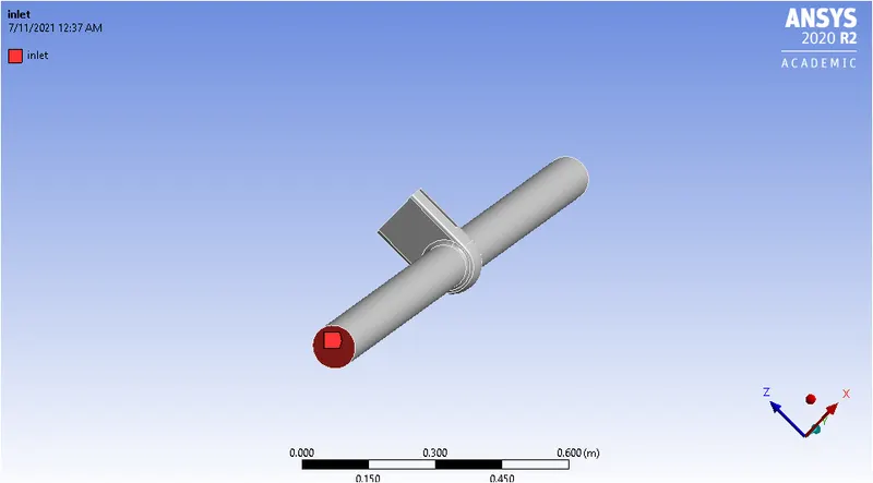
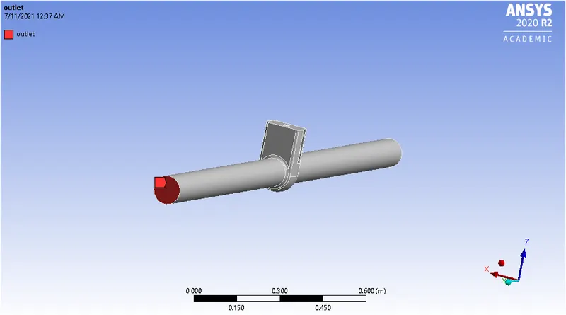
Creating named selection

Mesh

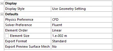
Open the meshing console and generate a mesh size of 0.01m

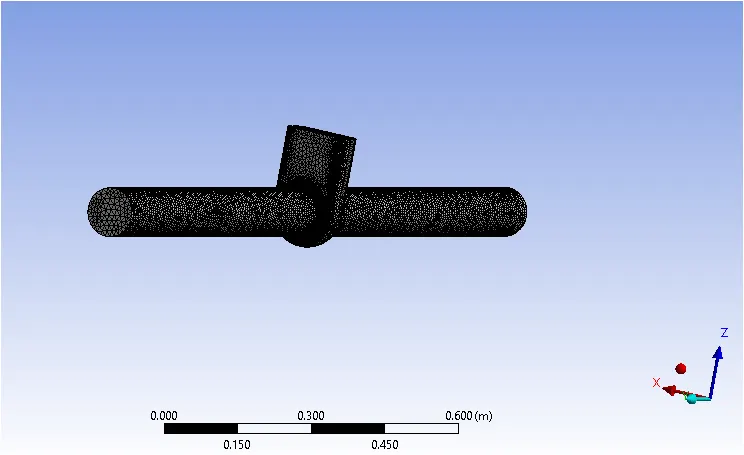
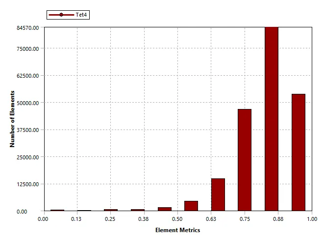
Ensuring mesh quality is above the required minimum level

Setting up physics

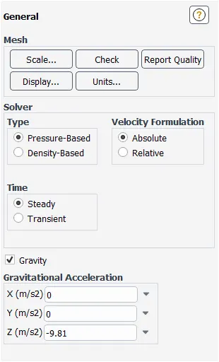
Solver Settings

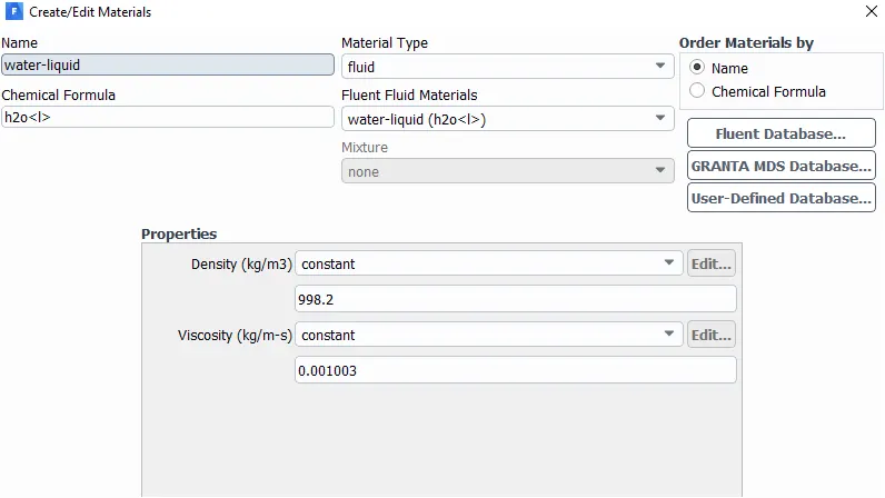
Material selection

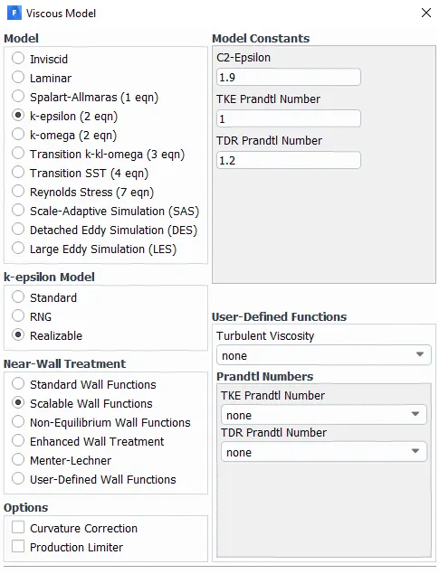
For turbulent model, select k-epsilon with realizable and scalable wall function

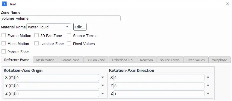
Selection of water as material for fluid flow.

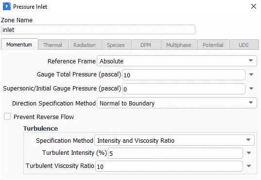
Applying boundary conditions

For inlet, we select pressure-inlet

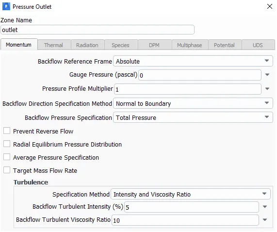
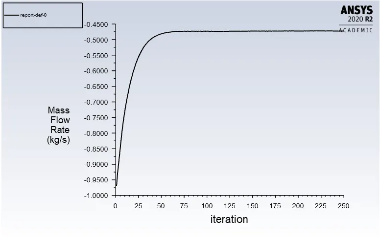
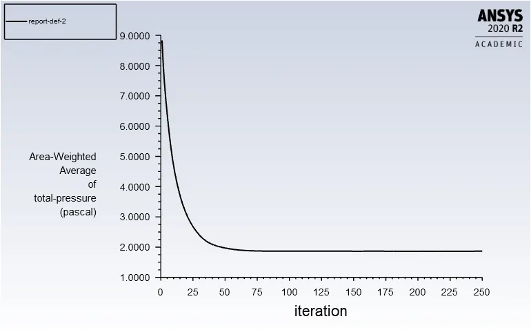
For report definition, select mass flow rate and total pressure at the outlet and select the option of create output parameter.

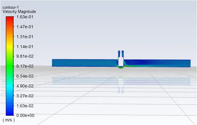
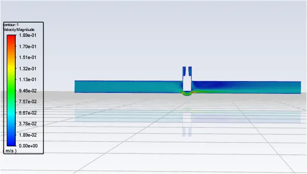
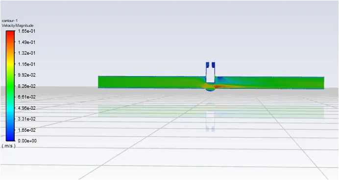
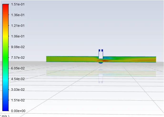
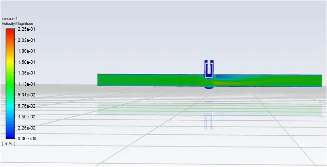
Creating a plane at a cross section of the gate valve and velocity contours to observe the flow of water.

We select standard initialization and initialize from the inlet.

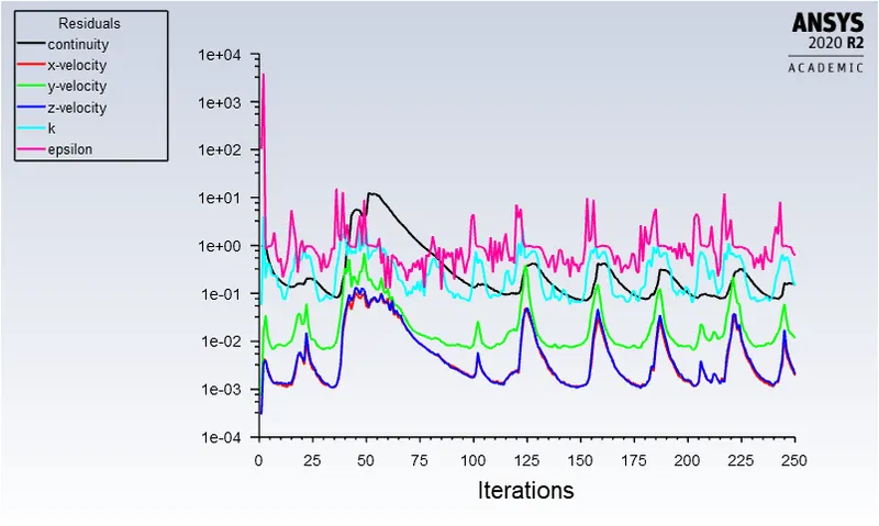
Run the simulation for 250 iterations.

Post processing at different points

Case 1

Gate disc lift = 10mm

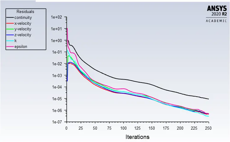
Residuals

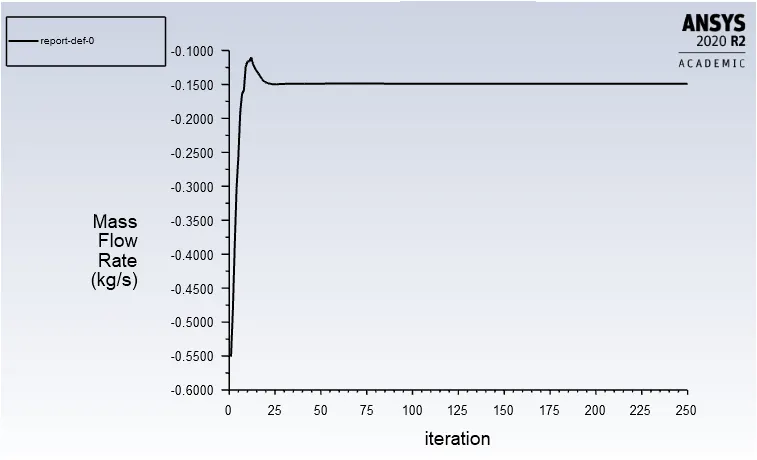
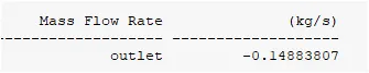
Mass flow rate

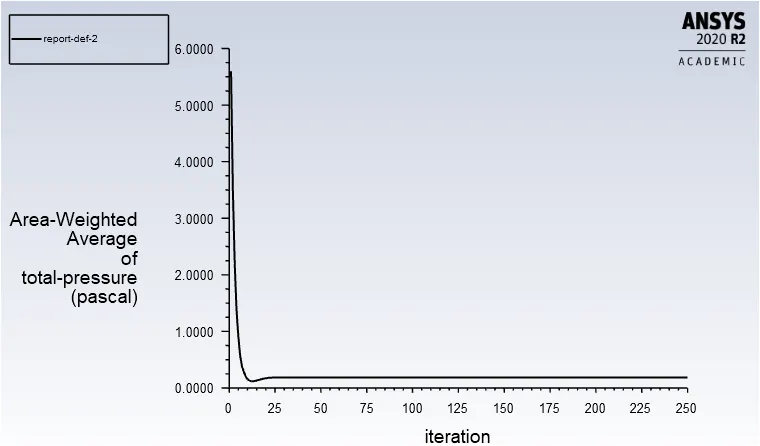
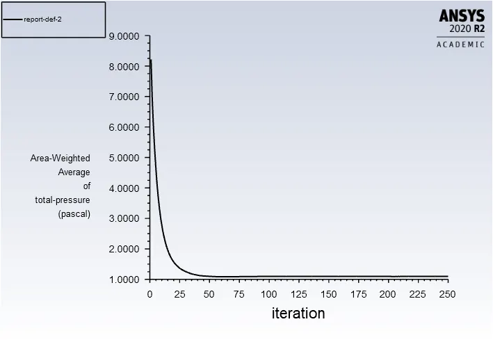
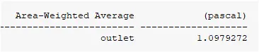
Pressure at the outlet

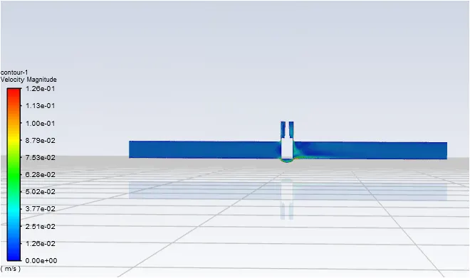
Case 2

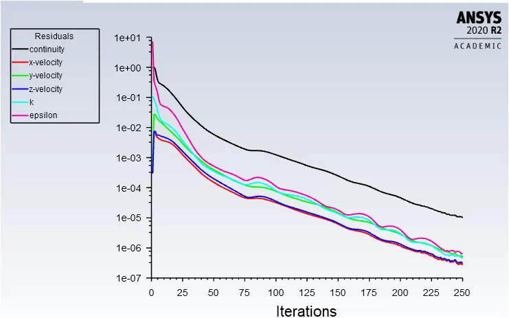
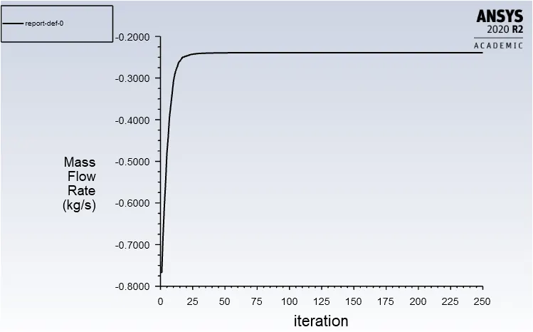
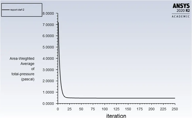
Gate disc lift = 20mm

Residuals

Mass flow rate

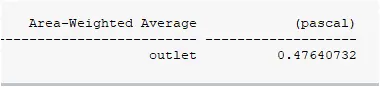
Pressure at the outlet

Case 3

Gate disc lift = 30mm

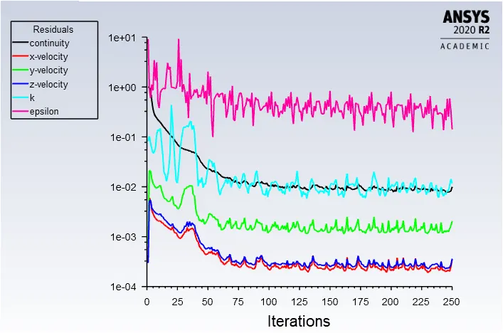
Residuals

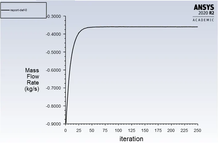
Mass flow rate

Pressure at the outlet

Case 4

Gate disc lift = 40mm

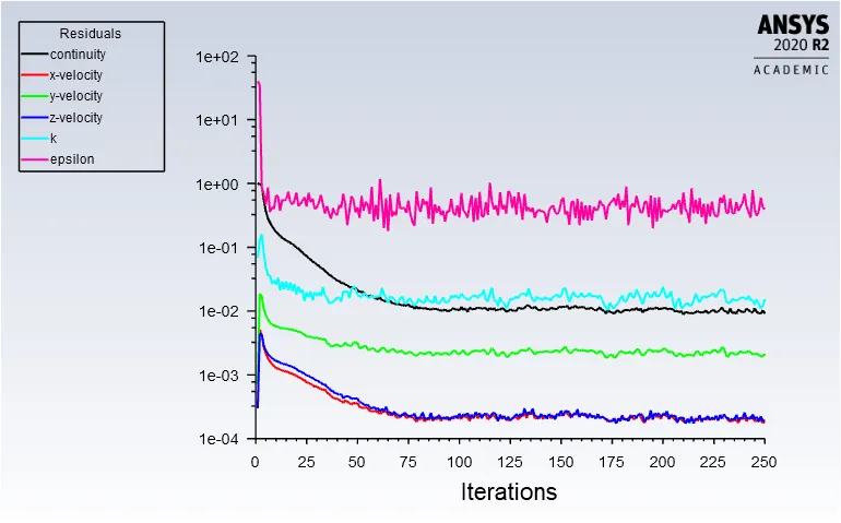
Residuals

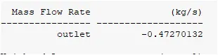
Mass flow rate

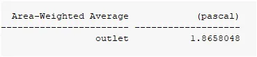
Pressure at the outlet

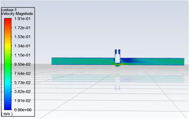
Case 5

Gate disc lift = 50mm

Residuals

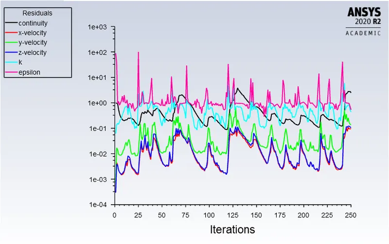
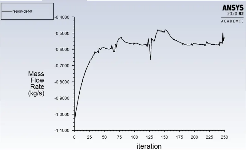
Mass flow rate

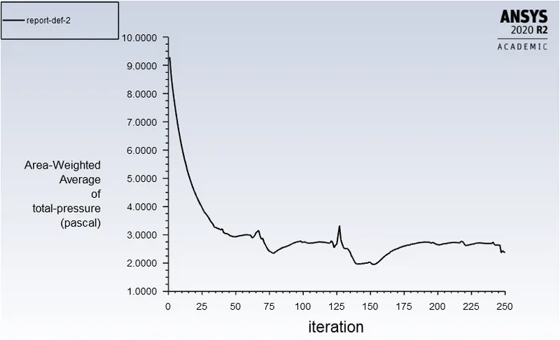
Pressure at the outlet

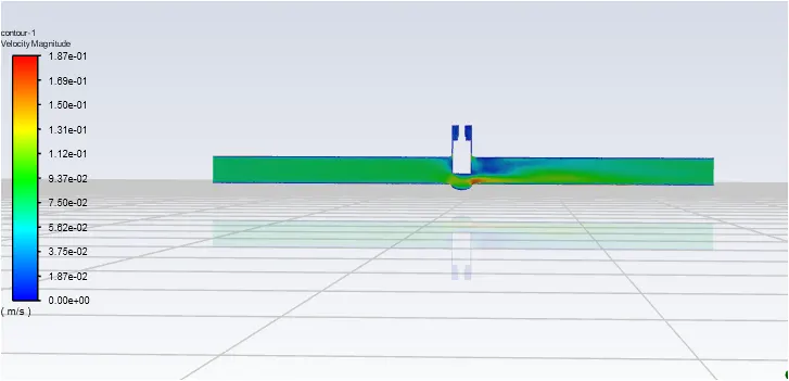
Case 6

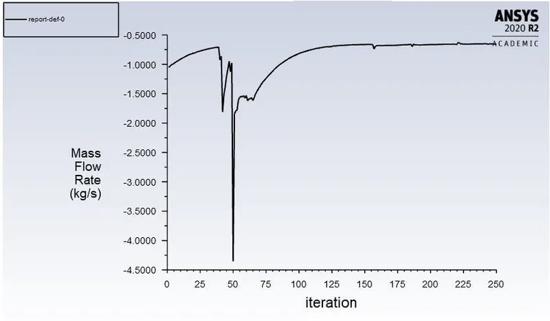
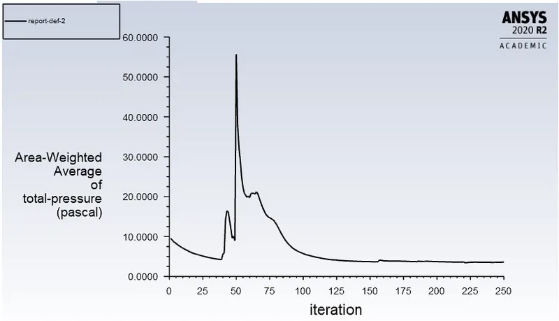
Gate disc lift = 60mm

Residuals

Mass flow rate

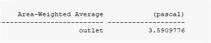
Pressure at the outlet

Case 7

Gate disc lift = 70mm

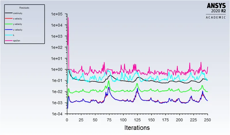
Residuals

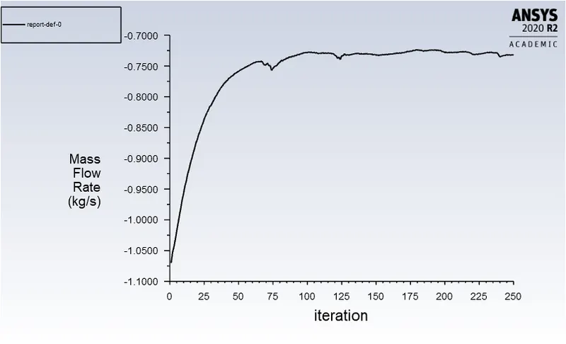
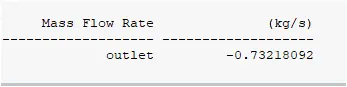
Mass flow rate

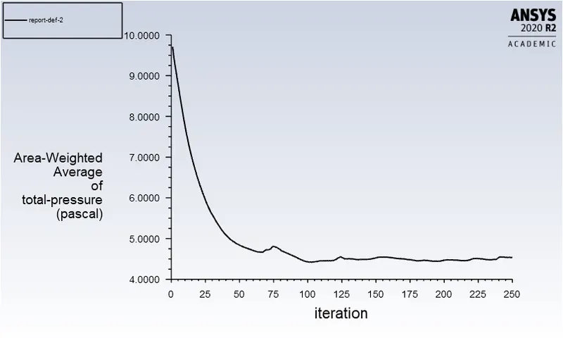
Pressure at the outlet

Case 8

Gate disc lift = 80mm

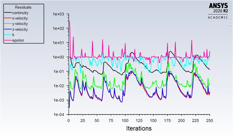
Residuals

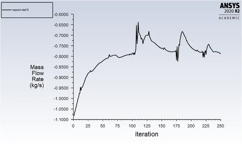
Mass flow rate

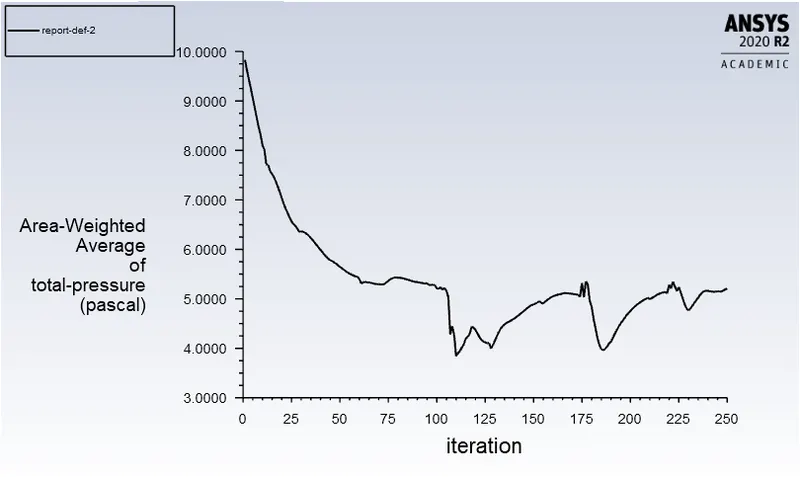
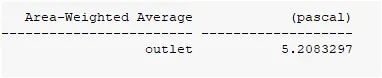
Pressure at the outlet

Flow coefficient (C_v )

The flow coefficient or C_v value is the number of US gallons of water the valve will pass with a differential pressure of 1psi through the valve at 60°F.

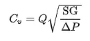
where,

Q is the rate of flow (gallons per minute)

SG is the specific gravity of the fluid (for water = 1)

ΔP is the pressure drop across the valve (expressed in psi).

Flow factor (K_v)

The K_v factor of a valve indicates the water flow in m³/h, at a pressure drop across the valve of 1 kgf /cm² when the valve is completely open.

K_v is the metric value of C_v and is calculated as K_v = C_v x 0.865.

Sr No	Lift Height (mm)	Mass flow rate (kg/s)	Mass flow rate (m3/h)	Mass flow rate (gallons/min)	Pressure inlet (Pa)	Pressure outlet (Pa)	Pressure drop (Pa)	Pressure drop (Psi)	Cv	Kv
1	10	0.1488	0.5356	2.3586	10	0.1852	9.8148	0.001423	62.5209	54.0805
2	20	0.2392	0.8611	3.7915	10	0.4764	9.5236	0.001381	102.029	88.2551
3	30	0.3604	1.2974	5.7125	10	1.0978	8.9022	0.001291	159.0008	137.5357
4	40	0.4727	1.7017	7.4926	10	1.8658	8.3142	0.001179	218.1681	188.7154
5	50	0.5322	1.9159	8.4357	10	2.3836	7.6164	0.001104	253.8418	219.5731
6	60	0.6565	2.3634	10.4059	10	3.5901	6.4099	0.000929	341.3282	295.2489
7	70	0.7322	2.6359	11.6058	10	4.5367	5.4633	0.000792	412.3494	356.6822
8	80	0.7877	2.8357	12.4855	10	5.208	4.792	0.000695	473.6587	409.7148

Conclusion

1. From the above table, it can be seen that flow coefficient and flow factor increases with increase in mass flow rate.
2. The negative mass flow rate at the outlet is due to the mass exiting the outlet.
3. The pressure drop decreases and mass flow rate increases with increase in lift height.