Week 6 - CHT Analysis on a Graphics card
Objective : To perform a steady-state conjugate heat transfer analysis on a model of a graphics card. To use appropriate materials for the simulation and making sure to properly define the correct solid and fluid zones.
- To run the simulation by varying the velocity from 1m/sec to 5m/sec for at least 3 velocities and discuss the results.
- Find out the maximum temperature and heat transfer coefficient attained by the processor.
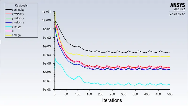
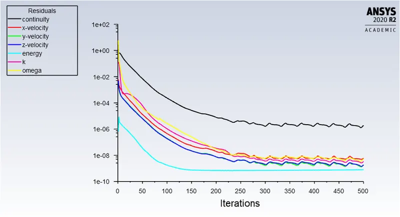
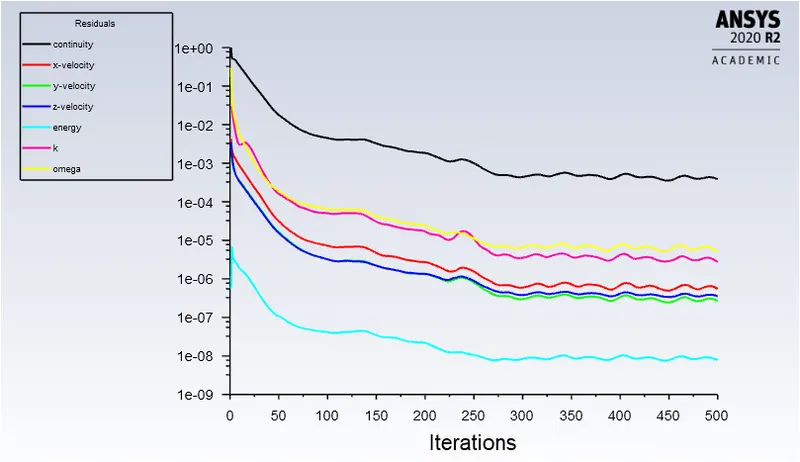
- Prove that the simulation has achieved convergence with appropriate images and plots.
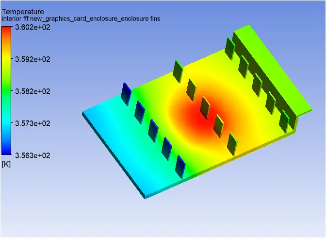
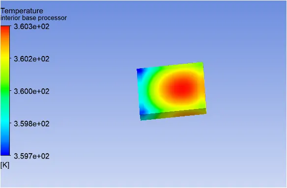
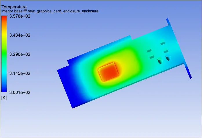
- Identify potential hotspots on the model.
Introduction
The Conjugate Heat Transfer (CHT) analysis type allows for the simulation of heat transfer between solid and fluid
Typical applications of conjugate heat transfer analysis are simulation of heat exchangers, cooling of electronic equipment, simulation of internal combustion engines, simulation of pumps and compressors and general-purpose cooling and heating systems.
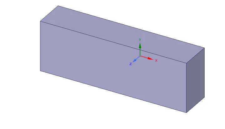
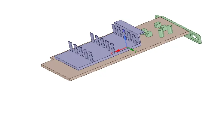
Geometry.
Using Spaceclaim to load the geometry.
Check for extra edges and interference in the geometry.
Use share topology between the different components so that information can be shared betwen different zones of the mesh.
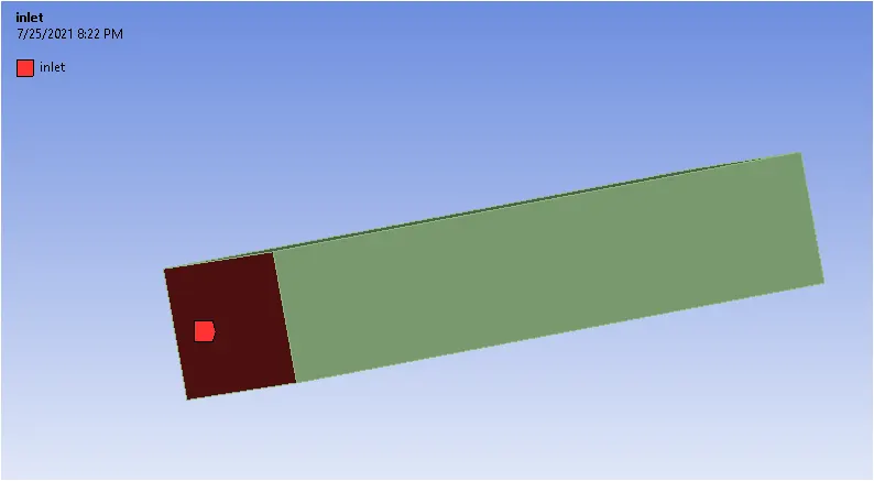
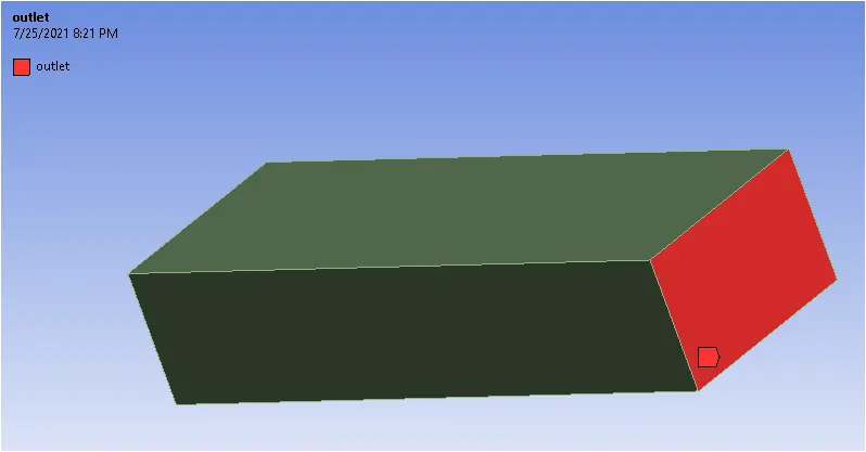
Creating Named selection
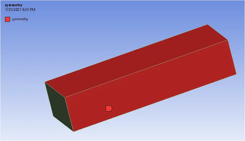
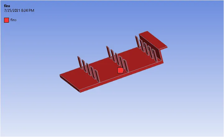
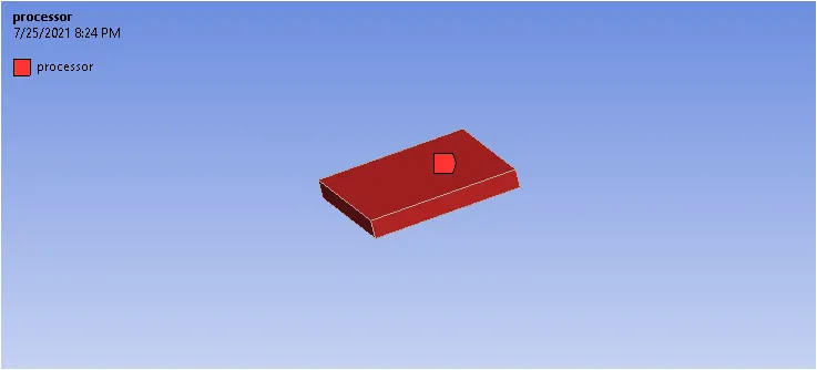
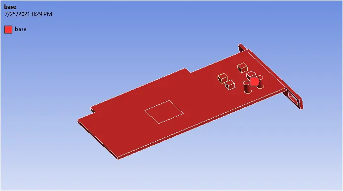
Mesh
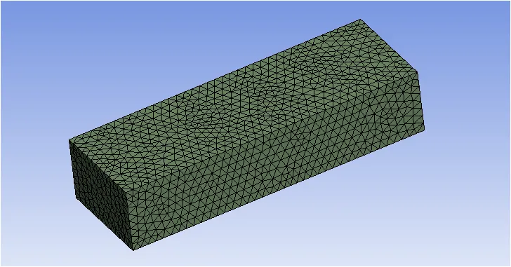
Generating a baseline mesh
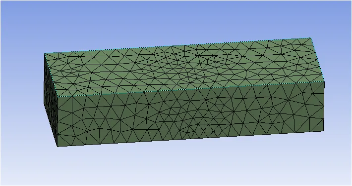
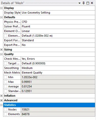
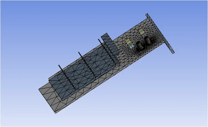
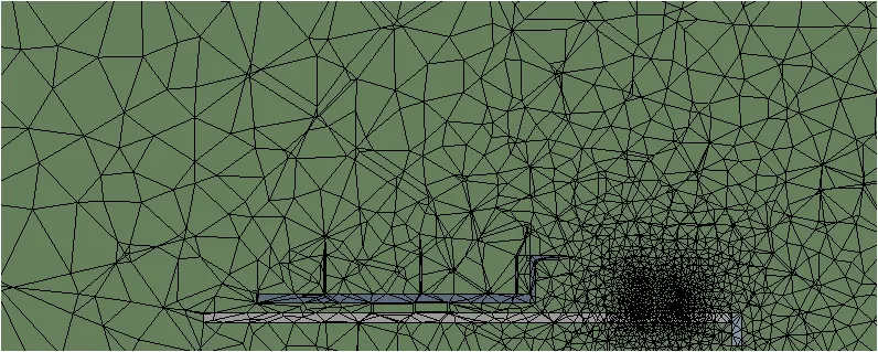
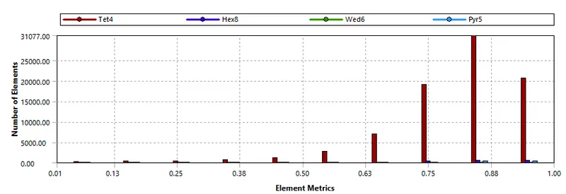
Ensuring most of the mesh elements are above the required quality
Setting up physics
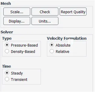
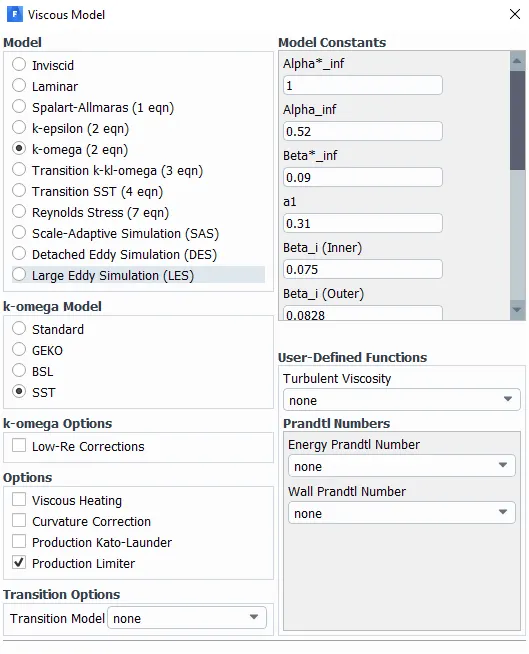
Selecting K-Omega SST as the turbulence model and keeping the energy equation on
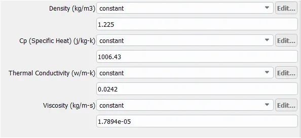
Material Selection
Different materials are used for different components
Fluid : Air
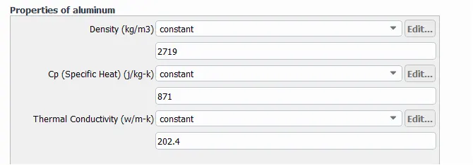
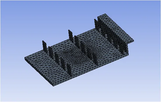
Fins : Aluminium
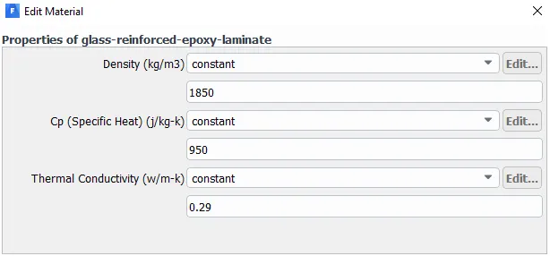
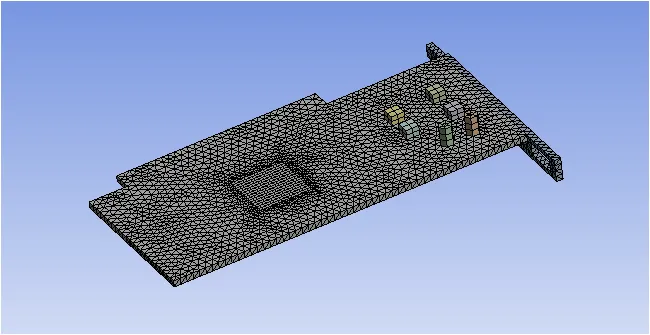
Base : FR4 (glass reinforced epoxy laminate)
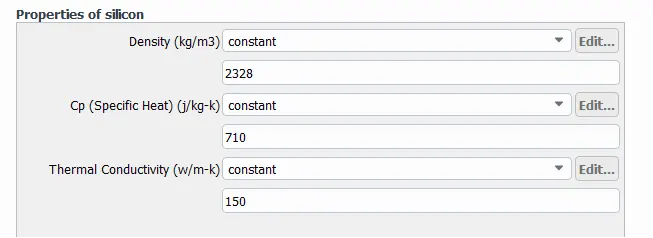
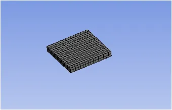
Processor : silicon
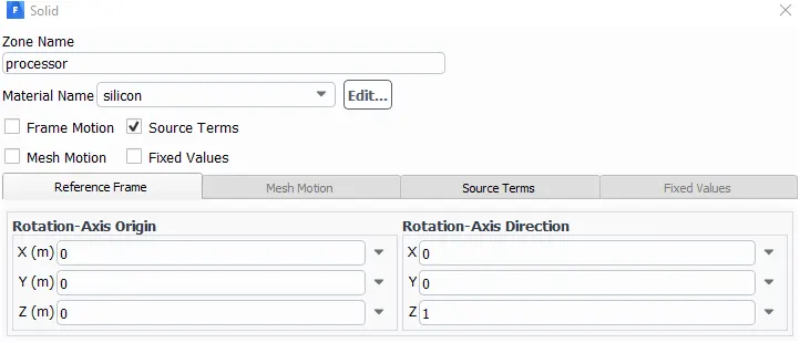
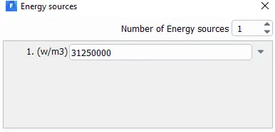
Setting up source term
Let the processor consume 2W of power.
Dimension of the processor = 64mm³
So the energy produced by the processor = 31250000W/m³
Inlet
Air is used as fluid
Velocity = 1m/s
Temperature = 300K
Outlet
Gauge pressure (0 pa)
Post Processing
Case 1
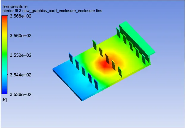
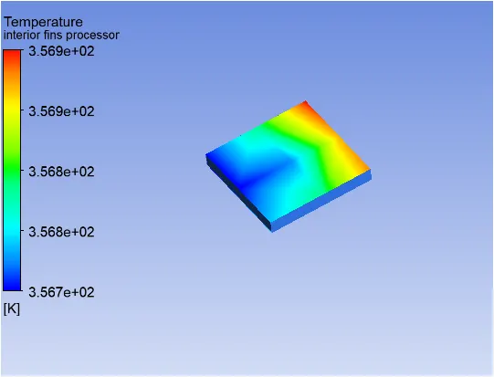
Base mesh with velocity of 1m/s
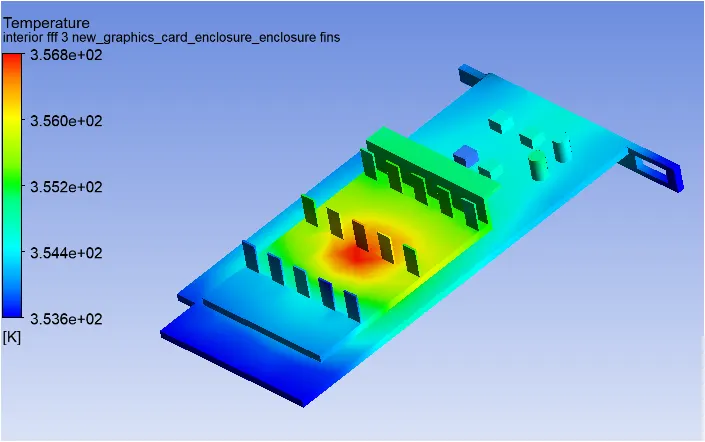
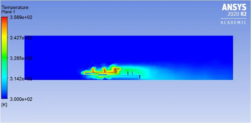
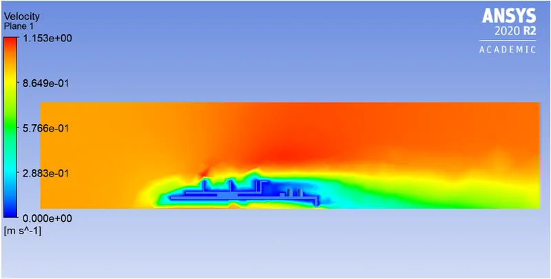
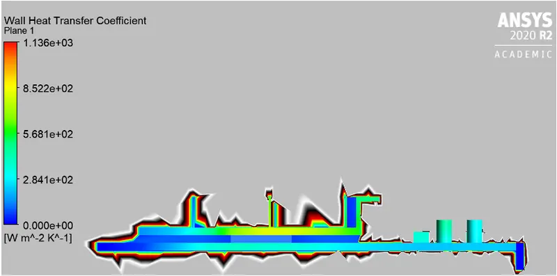
Hotspots
Refined mesh
Enclosure : 5mm
fins : 1mm
processor : 0.5mm
base : 1mm
Number of mesh elements : 197712
Case 2
Refined mesh with velocity of 1m/s
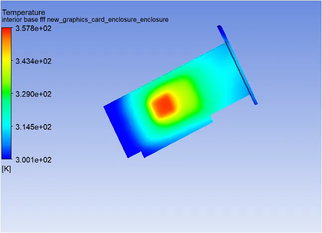
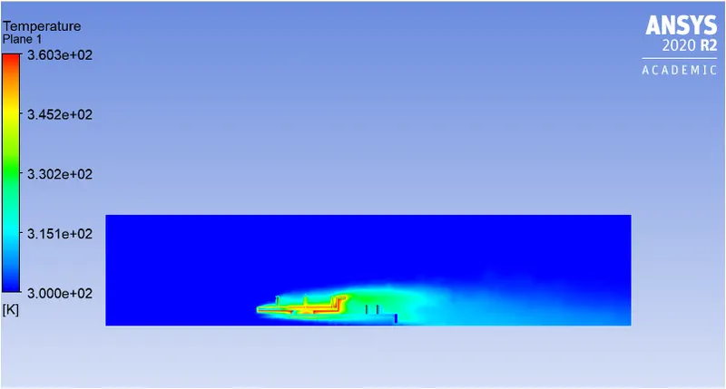
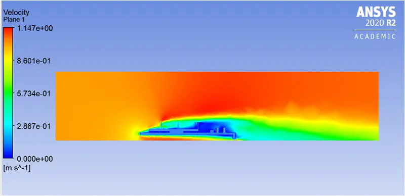
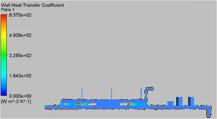
Hotspot
Case 3
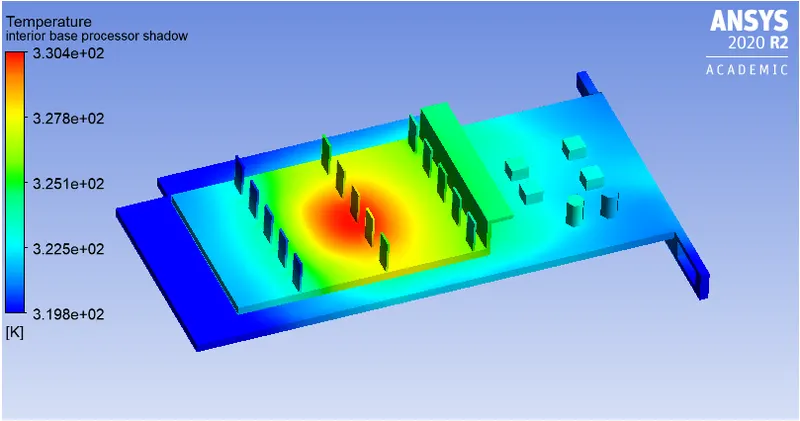
Refined mesh with velocity of 3m/s
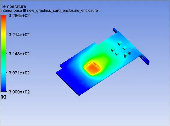
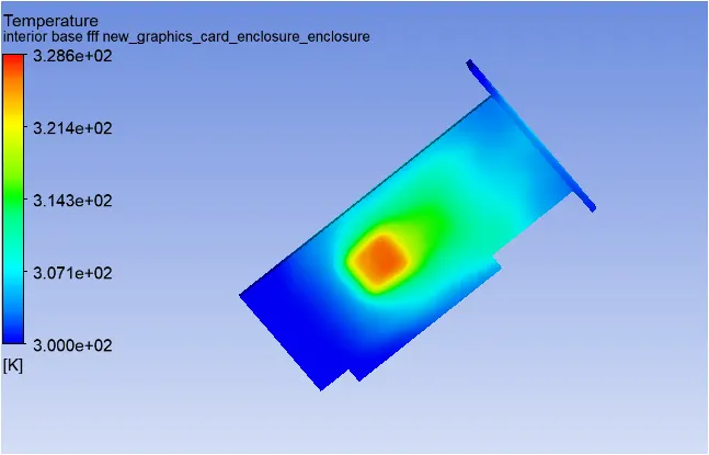
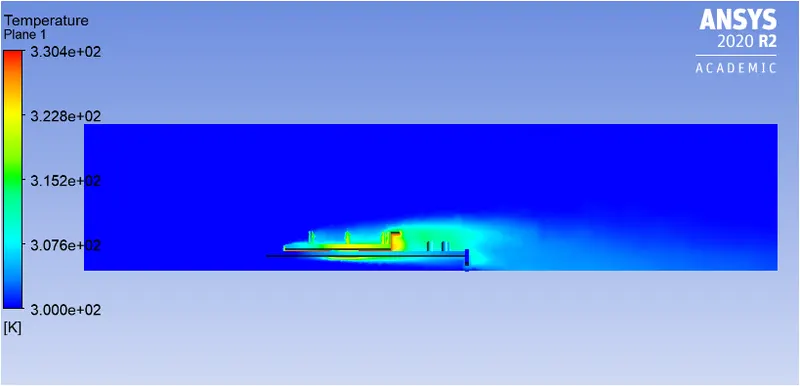
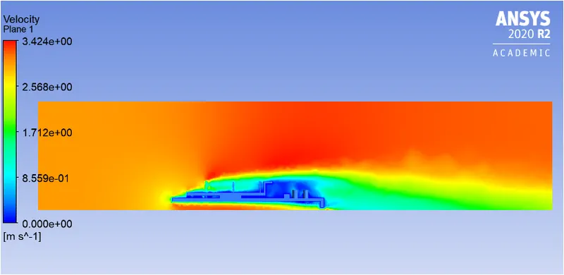
Hotspot
Case 3
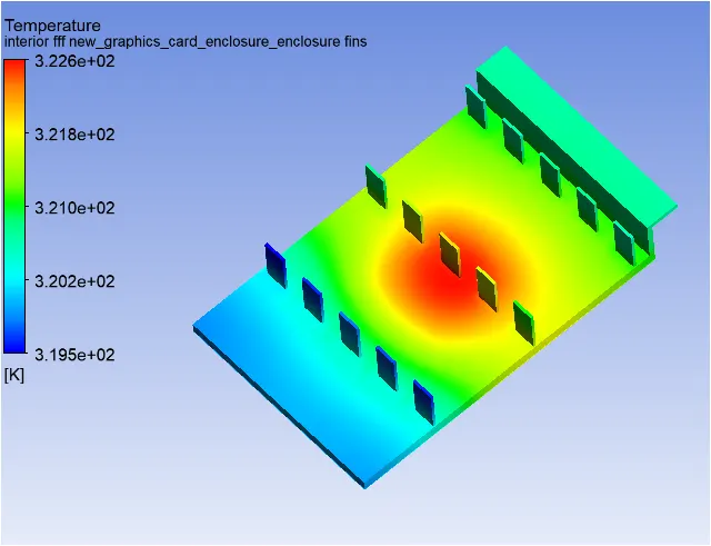
Refined mesh with velocity of 5m/s
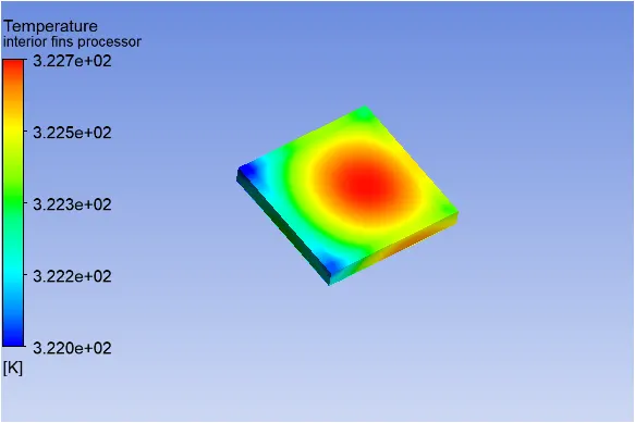
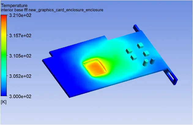
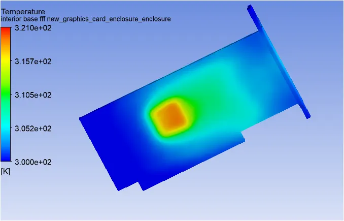
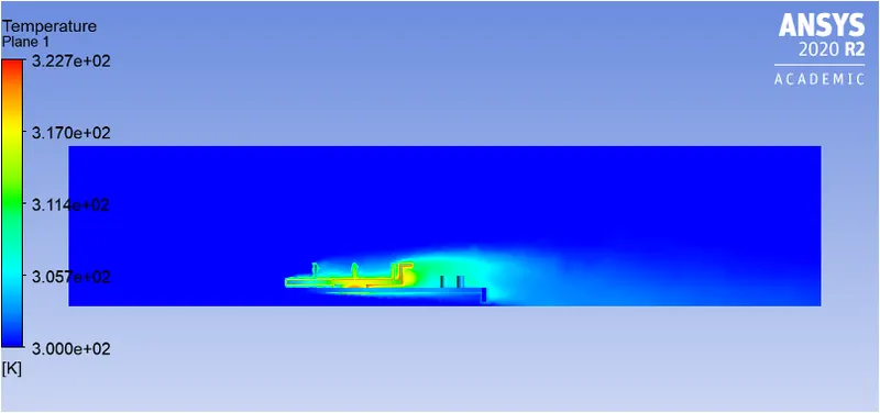
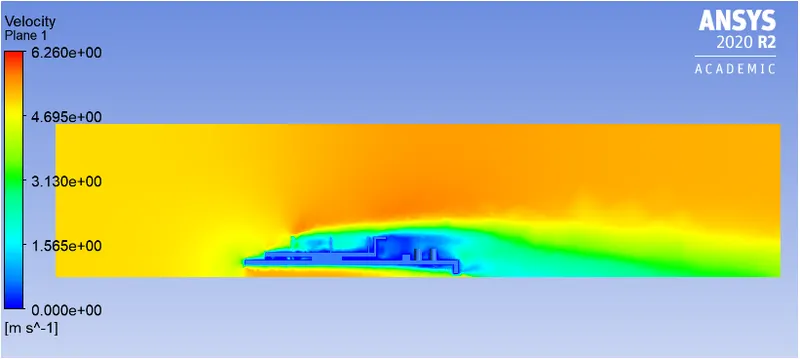
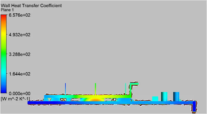
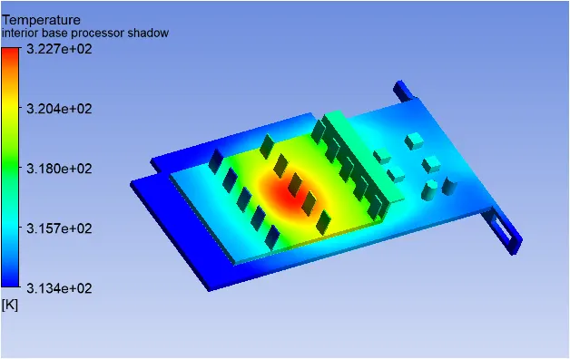
Hotspot
Results and Conclusion
| Sr No | Case | Velocity (m/s) | Max Temperature at processor (K) |
| 1 | Base mesh | 1 | 356.9 |
| 2 | Refined mesh | 1 | 360.3 |
| 3 | Refined mesh | 3 | 330.4 |
| 4 | Refined mesh | 5 | 322.7 |
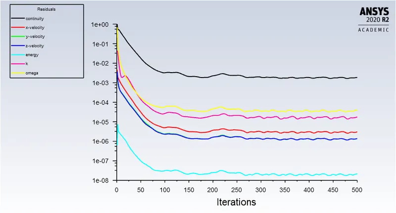
The values of all the residuals are below 1e-3 and are almost constant after 300 iterations. From the residuals plot, it can be said that the solution has converged.
As the number of mesh element increases, the results of the simulation becomes more accurate.
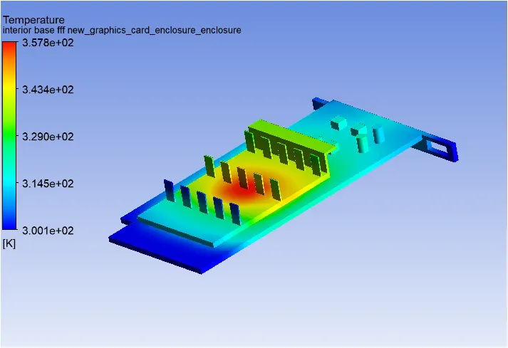
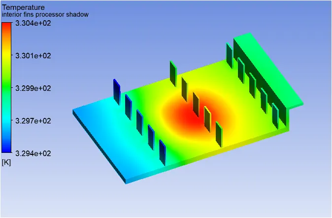
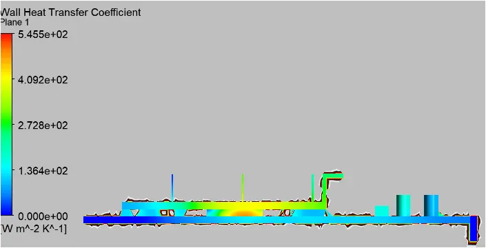
From the temperature contours of graphics card, it can be seen that the maximum temperature is obtained by the processor. The heat generated by the processor is conducted to the fins and then convected by the fins to the surroundings. Fins are surfaces that extend from an object to increase the rate of heat transfer to or from the environment by increasing convection. The fins which are closer to the processor have higher temperature while the fins which are away from the processor have lower temperature.
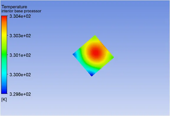
The major hotspot regions of the model are processor and the portion of base and fins which are in contact with the processor.
A small portion of heat is conducted through FR4 base. Since fins are made of aluminium which is a better conductor of heat, most of the heat generated by the processor is conducted to the fins.
The maximum temperature attained by the processor will vary depending on the velocity of the air. The maximum temperature of the processor decreases with increase in the velocity of air. Thus, it can be deduced that higher inlet velocity results in lower temperature of the components which helps in the components being safe from the effects of high temperature.