Week 5 - Rayleigh Taylor Instability

Objective

1. What are some practical CFD models that have been based on the mathematical analysis of Rayleigh Taylor waves? In your own words, explain how these mathematical models have been adapted for CFD calculations.
2. Perform the Rayleigh Taylor instability simulation for 2 different mesh sizes with the base mesh being 0.5 mm. Compare the results by showing the animations( Attach them from your google drive). Observe the differences in the animation and explain the effect of mesh size on simulation. Also, explain why a steady-state approach might not be suitable for these types of simulation.[ Choose Air and Water for this simulation]
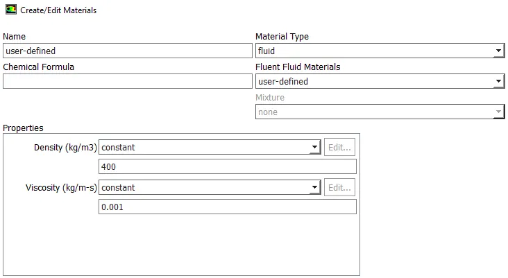
3. Run one more simulation with water and user-defined material(density = 400 kg/m³, viscosity = 0.001 kg/m-s) for refined mesh.
4. Define the Atwood Number. Find out the Atwood number for both the cases and explain how the variation in Atwood number in the above two cases affects the behavior of the instability.

Introduction

Fluid instabilities show up everywhere in nature. Fluid flow will start off laminar and smooth and then quickly transition to an irregular pattern eventually transitioning to turbulence.

Stratified fluid instabilities

From a fluid instability perspective, stratified fluid systems are in some ways the easiest to understand and visualize. It is often the case when there is a fluid system in which two fluids with different properties, an unstable configuration can be realized. In this case, there is a clear boundary between two fluids and this can be extended to a continuous variation between fluids, but the diffusion effects would damp out any perturbation and instability, so would not be as pronounced.

Buoyancy driven instabilities

Buoyancy-driven fluid instabilities occur in a stratified fluid system when the light fluid is accelerated into the heavier one often by means of a pressure gradient.

Some practical CFD models that have been based on the mathematical analysis of Rayleigh Taylor waves are:

Kelvin-Helmholtz instability

The Kelvin–Helmholtz instability typically occurs when there is velocity shear in a single continuous fluid, or additionally where there is a velocity difference across the interface between two fluids. A common example is seen when wind blows across a water surface, the instability constant manifests as waves.

Plateau–Rayleigh instability

The Plateau–Rayleigh instability explains why and how a falling stream of fluid breaks up into smaller packets with the same volume but less surface area. The driving force of the Plateau–Rayleigh instability is that liquids, by virtue of their surface tensions, tend to minimize their surface area.

Rayleigh-Taylor instability

The Rayleigh-Taylor instability is a buoyancy-driven instability where the acceleration is constant with respect to the fluid flow time. An important example of the Rayleigh-Taylor instability is when a heavy fluid lies atop a light one while in the presence of a downward acting gravitational field.

Richtmyer–Meshkov instability

The Richtmyer–Meshkov instability occurs when two fluids of different density are impulsively accelerated. Normally this is done by the passage of a shock wave. The development of the instability begins with small amplitude perturbations which initially grow linearly with time. This is followed by a nonlinear regime with bubbles appearing in the case of a light fluid penetrating a heavy fluid, and with spikes appearing in the case of a heavy fluid penetrating a light fluid.

Geometry

Open spaceclaim in Ansys Fluent

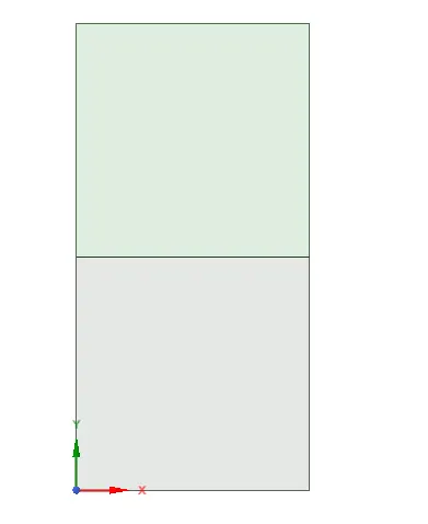
Create a square of 20 x 20mm. Use of pull tool to create a surface

Move the generated component to a new component and naming it as air

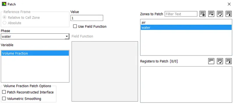
Draw a square of same size above this surface and naming it as water. It should be ensured that both the components are properly created.

Then go to workbench-share and select the geometry for sharing

Mesh

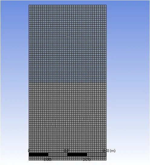
Open the meshing console and generate mesh of 0.5mm

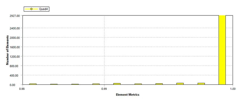
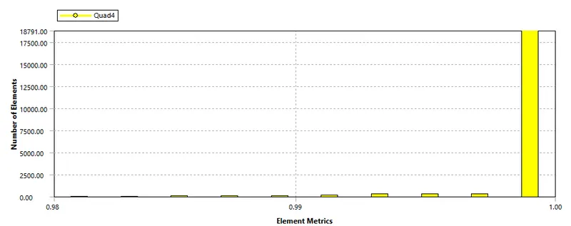
Ensuring mesh quality is above the minimum level

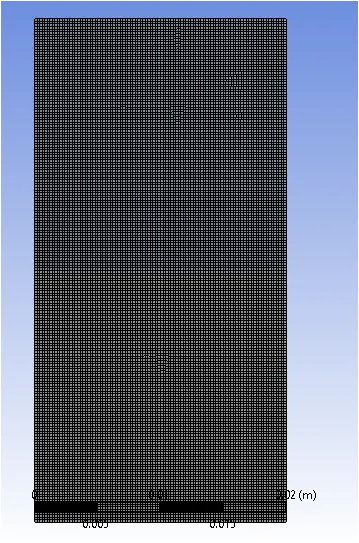
Refined mesh of 0.2mm

Ensuring mesh quality is above the minimum level for refined mesh

Setting up physics

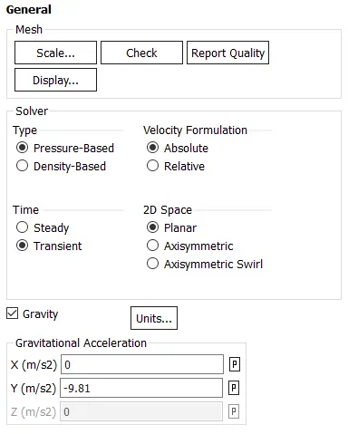
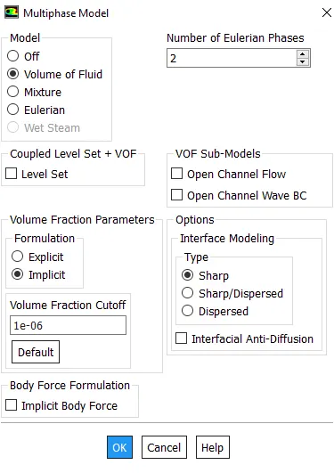
After updating mesh, selection of solver

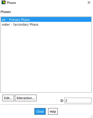
Material Selection

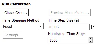
Post processing and Results

Case 1

Mesh size : 0.5mm

Materials : air and water

Residuals

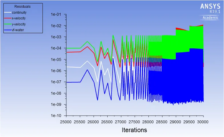
Steady state plot

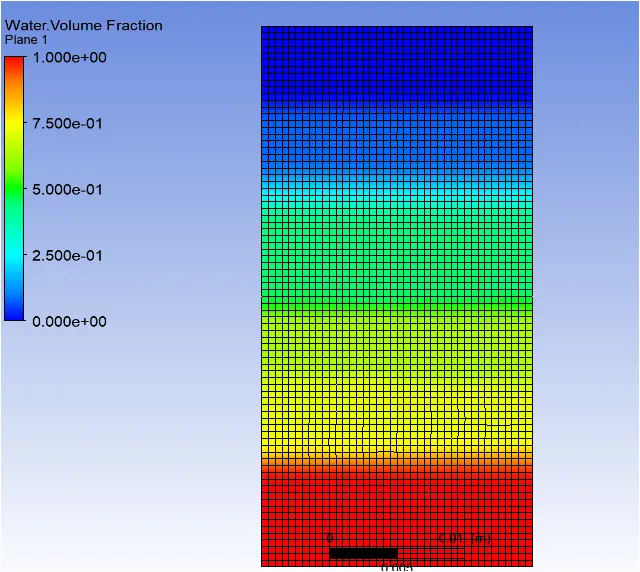
Animation Google drive link

https://drive.google.com/file/d/1Kj_h4b8epiDP6wACEQ7Li2v8W7HdVNOD/view?usp=sharing

Case 2

Mesh size : 0.2mm

Materials : air and water

Residuals

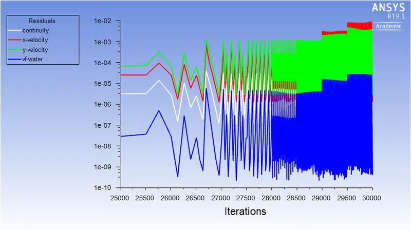
Steady state plot

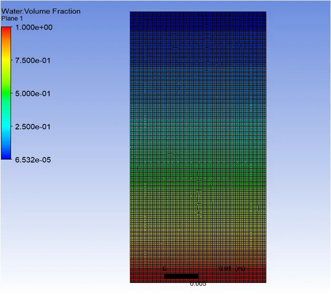
Animation Google drive link

https://drive.google.com/file/d/18BQXGtL8E60UKfYh6_E3KYpBI3QqIbUt/view?usp=sharing

Case 3 :

Mesh size : 0.2mm

Materials : user-defined and water

Residuals

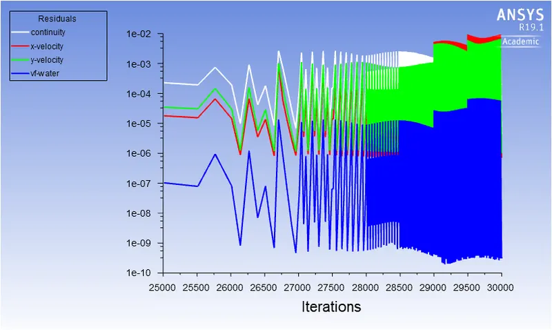
Steady state plot

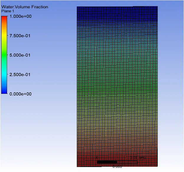
Animation Google drive link

https://drive.google.com/file/d/1rc_vJaPwe81nv8pXayZJ4O85BVW99hfa/view?usp=sharing

Atwood Number

The Atwood number (A) is a dimensionless number in fluid dynamics used in the study of hydrodynamic instabilities in density stratified flows. It is a dimensionless density ratio defined as

where

A is the Atwood number

ρ₁= density of heavier fluid

ρ₂ = density of lighter fluid

Case 1

For fluids water and air

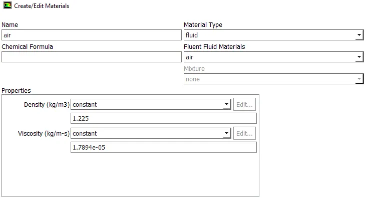
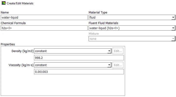
ρ₁= density of water = 998.2 kg/m³

ρ₂ = density of air = 1.225 Kg/m³

A = (998.2-1.225)/(998.2+1.225) = 0.9975

Case 2

For fluids water and user defined

ρ₁= density of water = 998.2 kg/m³

ρ₂ = density of user defined fluid = 400 Kg/m³

A = (998.2-400)/(998.2+400) = 0.4278

Conclusion

In case of smaller Atwood number, the density difference of the fluids on either side of the interface is small and the density distribution of the upper and lower layers is symmetrical. In case of larger Atwood number, the density difference of the fluids on either side of the interface is large. In this case, the two edges of the mixing layer develop into spikes on the light fluid side and bubbles on the heavy fluid side. The bubbles and spikes appears at a larger rate for high Atwood number cases.

In Rayleigh Taylor instability simulation, fine mesh helps to capture instability more accurately than coarse mesh. The time required for settling of fluid is more in fine mesh as compared to coarse mesh.

The difference between steady state and transient simulation is that in steady state case, the intermediate variables/parameters as a function of time cannot be observed/determined. The steady state simulation is used only if we require final state solution irrespective of intermediate states. In Rayleigh Taylor instability problem, we are interested in observing the transition of the irregularities when high density fluid is placed on low density fluid under the influence of gravity. Hence, we are interested in observing the instabilities occurring at different instants of time during the course of simulation and not only on end result. The final state results for both steady and transient simulation will be the same.