Week 2 - Flow over a Cylinder.
Objective : To simulate the flow over a cylinder and understanding the phenomenon of Von Karman vortex street.
To simulate the flow with the steady and unsteady case and calculate the Strouhal Number for Re= 100.
To calculate the coefficient of drag and lift over a cylinder by setting the Reynolds number to 10,100,1000,10000 & 100000.
To determine the effect of Reynolds number on the coefficient of drag.
Geometry
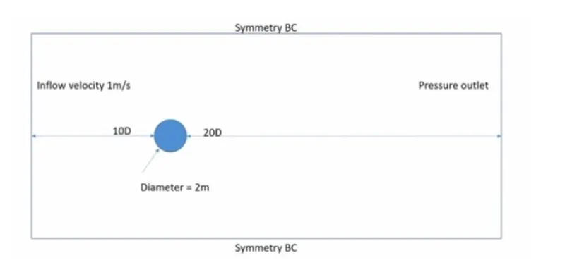
The computational domain required for the simulation is created in spaceclaim. The dimensions of the geometry are as follows :
Boundary naming
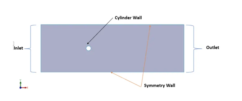
After the creation of computational domain for the simulation, appropriate boundary names were assigned to carry out the simulation smoothly. For the purpose of this simulation, four boundary names are assigned. They are inlet, outlet, cylinder wall and symmetry walls. These boundaries are shown in the below figure :
Meshing
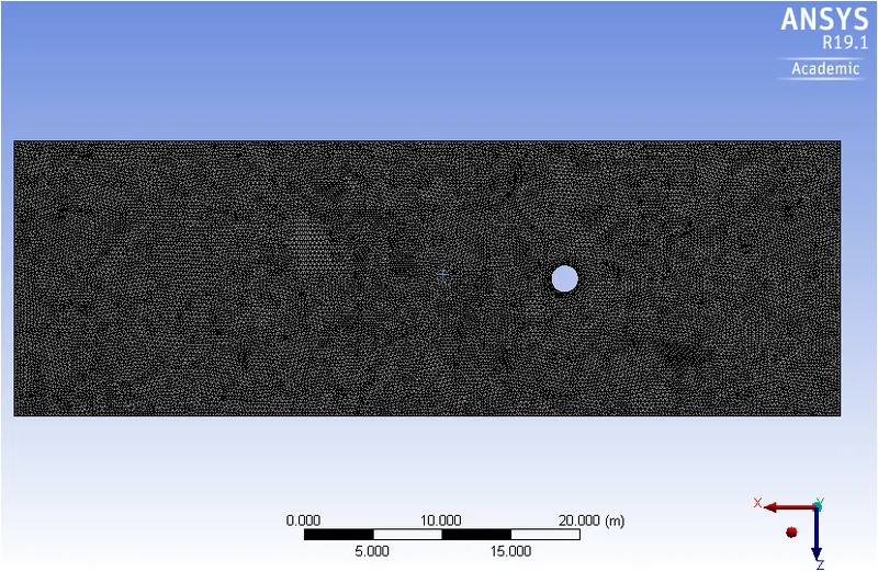
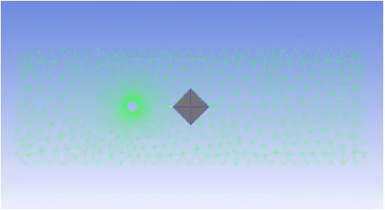
For this simulation, triangular mesh was chosen as the type of mesh element. The size of the mesh element is 0.25m. The meshing of the geometry is as follows :
Inflation layer
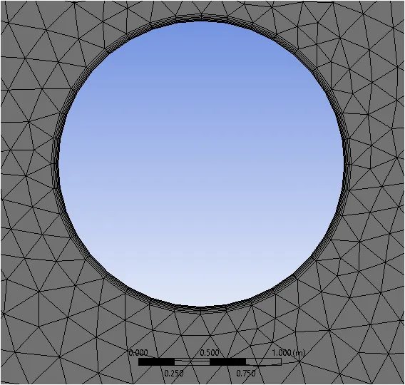
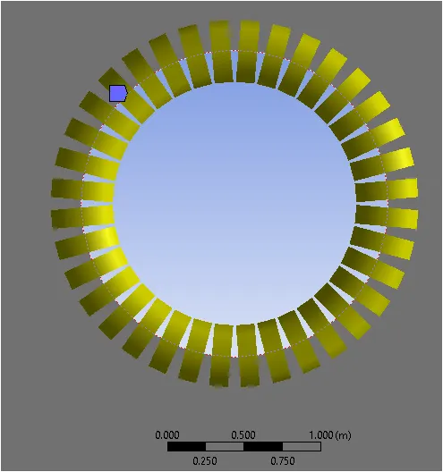
Inflation layers were used in order to make the mesh more refined near the walls to capture the flow properties around the cylinder more accurately. The number of inflation layers used were 6 with a growth rate of 1.2
Edge sizing
Edge sizing was used around cylinder wall so that the circular property of cylinder wall is not distorted. The number of divisions used in edge sizing were 36.
Case setup
In setup, the type of solver used for simulation is pressure based solver. For steady flow, the type of time based solver used is steady and for unsteady flow, the type of time based solver used is transient. The type of viscous model used is laminar viscous model as the Reynolds number for the simulation is small. The material used for this simulation has a density of 1 kg/m3 and dynamic viscosity of 0.02 kg/m-s. SIMPLE scheme was used for solving the equations.
A monitor point was created behind the cylinder to capture the velocity at that point.
Results
Steady flow
The simulation was run for 500 iterations so that complete flow is captured.
Residuals plot
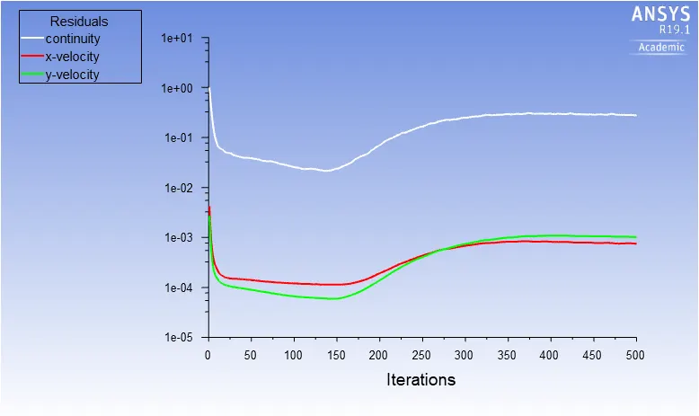
For this simulation, the residual plots are converged at around 400 iterations
Velocity monitor point
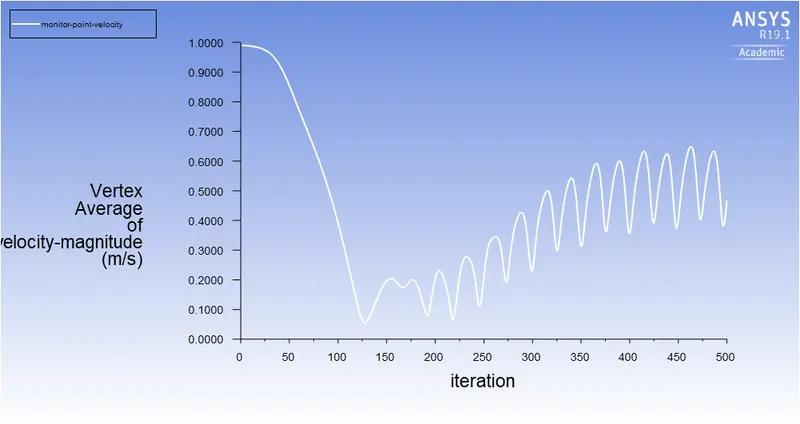
From the above graph, it can be seen that the velocity drops till 125th iteration and then shows wavy pattern due to vortex shedding. This is because the monitor point is a point behind the cylinder where vortex shedding happens.
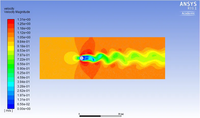
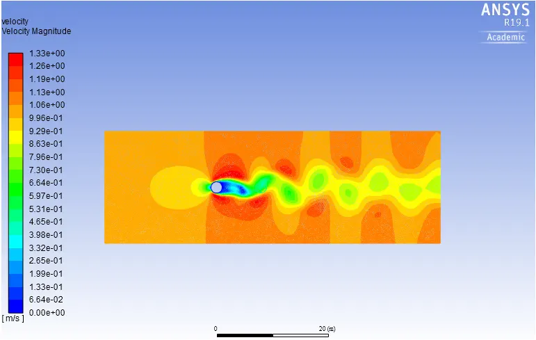
Vortex shedding is an oscillating flow that takes place when a fluid flows past a bluff body at certain velocities, depending on the size and shape of the body. In this flow, vortices are created at the back of the body and detach periodically from either side of the body. The fluid flow past the object creates alternating low-pressure vortices on the downstream side of the object.
Von Karman vortex street is a repeating pattern of swirling vortices, caused by vortex shedding which is responsible for the unsteady separation of flow of fluid around blunt bodies.
Velocity Contour
Transient flow
The simulation is run for 2000 time steps with a time step of 0.1s
Residuals plot
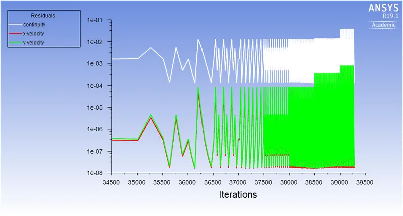
In transient flow, all the residuals have large oscillations and hence they do not get stabilized.
Monitor point velocity
Plot as a function of number of iterations
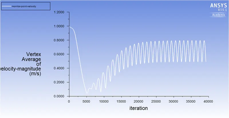
The vortex starts forming at around 7500 iterations and then gets stabilized at around 20000 iterations
Plot as a function of flow-time
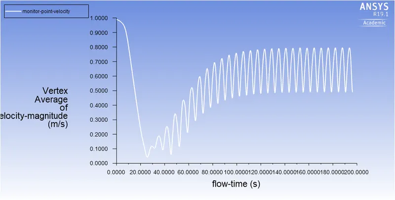
The vortex starts forming at around 30 seconds and then gets stabilized at around 100 seconds
Calculation of Strouhal number
The Strouhal number is a dimensionless number which represents the ratio of inertial forces due to the local acceleration of the flow to the inertial forces due to the convective acceleration.
Strouhal number = fL/U
Here,
f is the frequency of the oscillations
L is the characteristic length of the body
U is the flow velocity
For this simulation
Flow velocity (U) = 1 m/s
Characteristic length is the diameter of the cylinder (L) = 2m
Calculating number of oscillations between 100s and 180s
Frequency (f) = No of oscillations/Time = 13.5/80 = 0.16875
Strouhal number = fL/U = 0.16875*2/1 = 0.325
Velocity contour plot
Study of Lift coefficient and Drag coefficient over the cylinder when Reynolds number is changed.
In order to change the Reynolds number, value of flow velocity is changed to get different values of Reynolds number.
| Sr No | Reynold Number | Velocity |
| 1 | 10 | 0.1 |
| 2 | 100 | 1 |
| 3 | 1000 | 10 |
| 4 | 10000 | 100 |
| 5 | 100000 | 1000 |
Diameter of the cylinder =2m
Density = 1 kg/m3
Dynamic viscosity = 0.02 kg/m-s
The results for all the cases were generated using steady state simulation for 500 iterations.
Reynolds number = 10
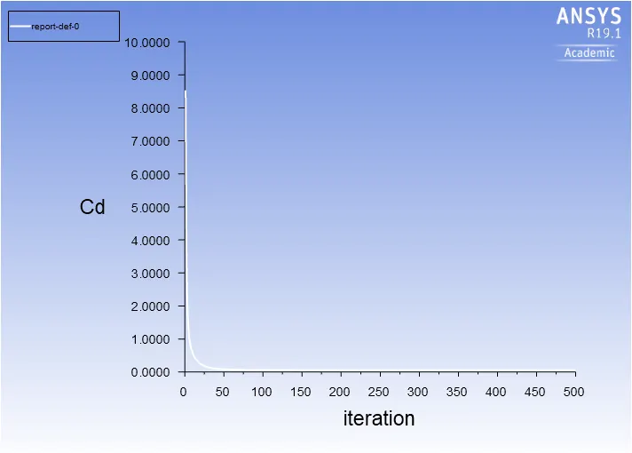
Drag coefficient
The average value of drag coefficient is 0.0543
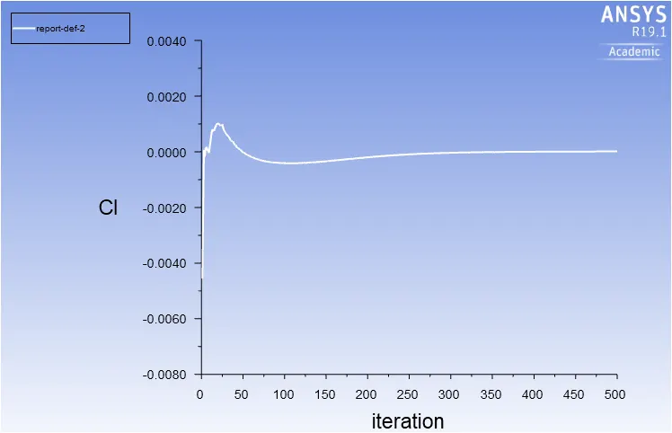
Lift coefficient
The average value of lift coefficient is 1.402e-5
Reynold number = 100
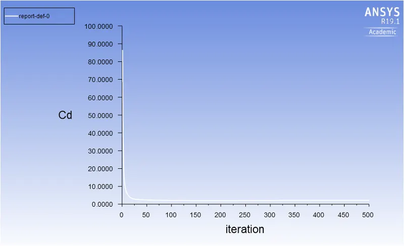
Drag coefficient
The average value of drag coefficient is 2.178
Lift coefficient
The average value of lift coefficient is -0.0945
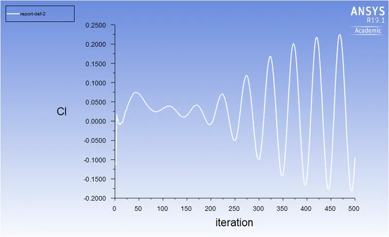
Reynolds number = 1000
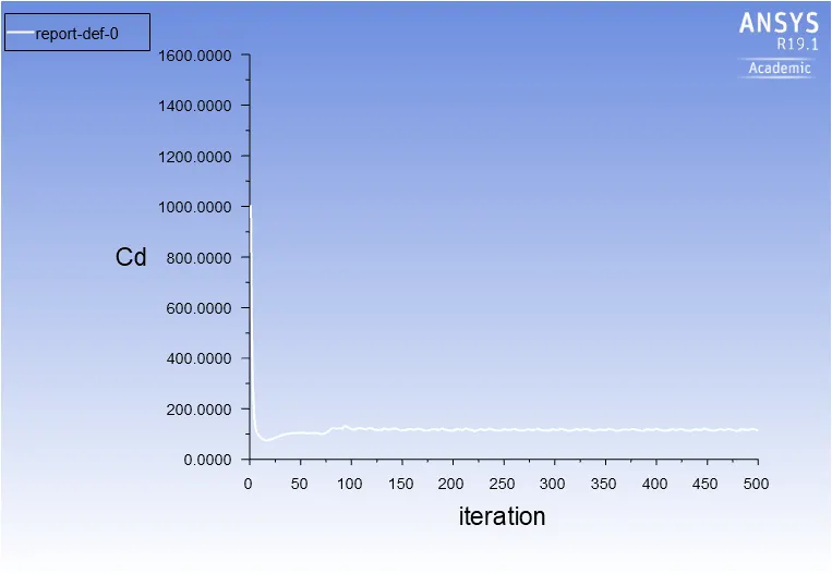
Drag coefficient
The average value of drag coefficient is 114.794
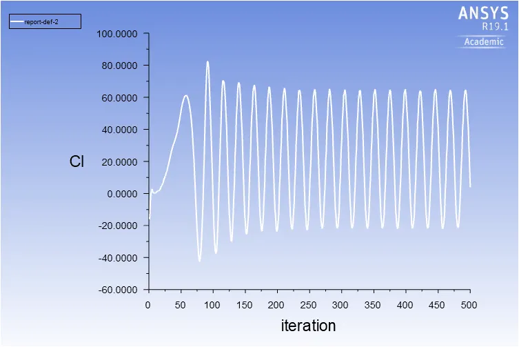
Lift coefficient
The average value of lift coefficient is 3.9366
Reynold number = 10000
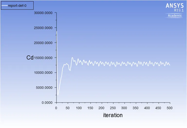
Drag coefficient
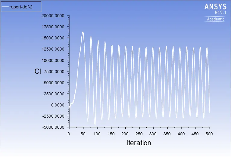
The average value of drag coefficient is 12385.343
Lift coefficient
The average value of lift coefficient is -1823.9537
Reynolds number = 100000
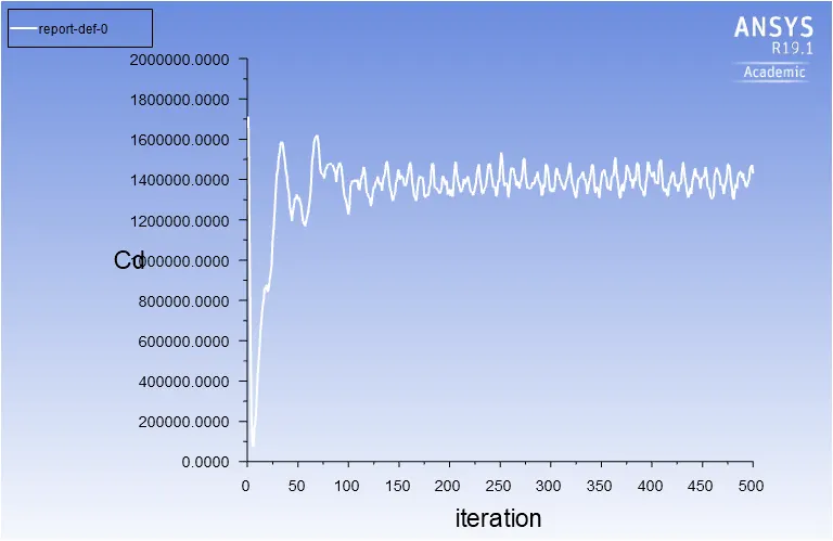
Drag coefficient
The average value of drag coefficient is 1429613.9
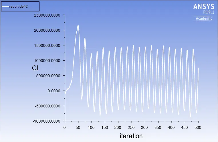
Lift coefficient
The average value of lift coefficient is 761303.06
Conclusions
1) Vortex shedding is observed in both steady and transient cases but the results of simulation from transient solver tends to be more accurate.
2) The number of iterations required for steady flow is less than that required for transient flow.
3) Strouhal number calculation is possible only for transient flow simulation only. This is because the frequency of vortex shedding cannot be determined in steady flow as there is no relation between velocity and flow time.
4) The drag coefficient increases with increase in Reynolds number.
Materials referred
Numerical simulation of laminar flow past a circular cylinder - B.N.Rajani. A. Kandasamy, Sekhar Majumdar
Viscous Fluid Flow - Nikolas D. Katopodes, in Free-Surface Flow, 2019