Week 1- Mixing Tee

Objective :To set up steady-state simulations for both shorter and longer mixing tee and to compare the mixing effectiveness when hot inlet temperature is 36⁰C & the Cold inlet is at 19⁰C.

1. Case 1
   • Short mixing tee with a hot inlet velocity of 3m/s.
   • Momentum ratio of 2, 4.
2. Case 2
   • Long mixing tee with a hot inlet velocity of 3m/s.
   • Momentum ratio of 2, 4.

Momentum ratio = velocity at cold inlet / velocity at hot inlet

CAD Model

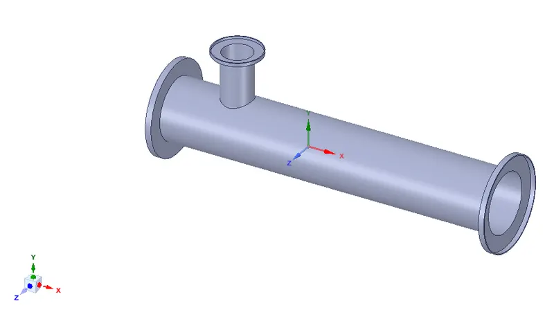
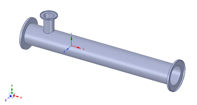
CAD Model for short and long mixing tee are as follows :

Short mixing tee

Long mixing tee

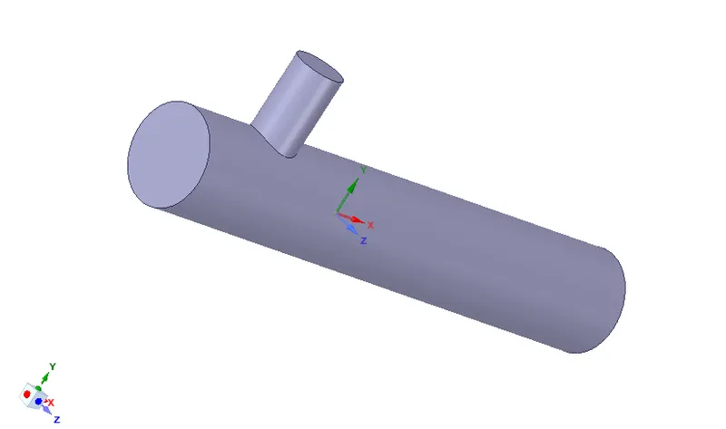
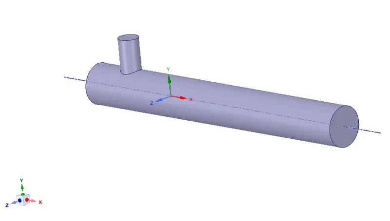
The above models are the given models. We need to convert this model as per the requirement of simulation. For this simulation, only those sections where fluid flow happens are required. So we use volume extraction option to get the required fluid flow region. After volume extraction, the models are as follows :

Short Mixing tee

Long Mixing tee

The next step of simulation is mesh generation.

All the faces are named in order to make the simulation easy in later stages.

Here, the hot fluid enters through inlet x and cold fluid enters through inlet y.

Mesh Generation

Mesh is generated for the above models with element size of 0.0015m or 1.5mm.

Mesh profile

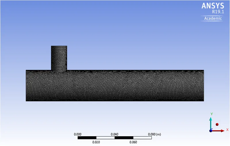
For getting appropriate results in simulation, it is necessary to get good quality mesh.

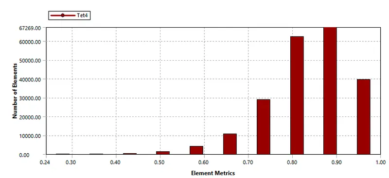
Here, the mesh quality is above 24% which can be used to get appropriate results in simulation.

Solver

Here, Ansys fluent is used for solving the simulation. Initially quality of mesh is checked. In setting up physics, steady state solver is used as we are interested only in final solution. Pressure based solver is used as Mach number for the given problem is less than 0.3. Velocity formation is taken as absolute. The viscous model selected for this problem is turbulence model. After this, boundary conditions are defined as per the requirement of this simulation.

The problem is initialized using hybrid initialization and the problem is run for required number of iterations depending on different cases. Since we require temperature at the outlet, the reports are generated for weighted average temperature and standard deviation of temperature at the outlet.

Mesh independence study

Three different mesh elements were selected and their effect on standard deviation of temperature and weighted average temperature at the outlet was determined.

Sr No	Mesh Element Size	Number of mesh elements	Weighted average temperature at outlet (Kelvin)	standard deviation of temperature at outlet
1	1.5mm	214218	303.54	1.984
2	1.3mm	303591	303.53	1.983
3	1.15mm	411420	303.53	1.983

From the above table it can be seen that with decrease in mesh size, there is almost no change in standard deviation of temperature and weighted average temperature at the outlet. Hence, it can be said that the simulation is mesh independent at element size of 1.5mm and all the further simulations are performed using this mesh size.

Results

Case 1: Short mixing tee with momentum ratio 2

k-omega SST model

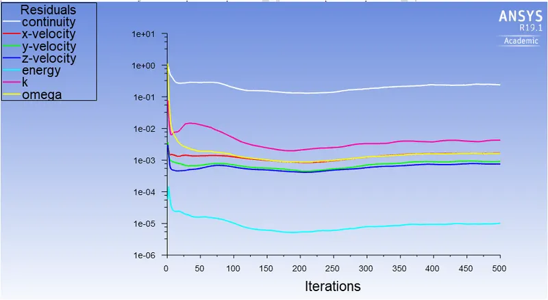
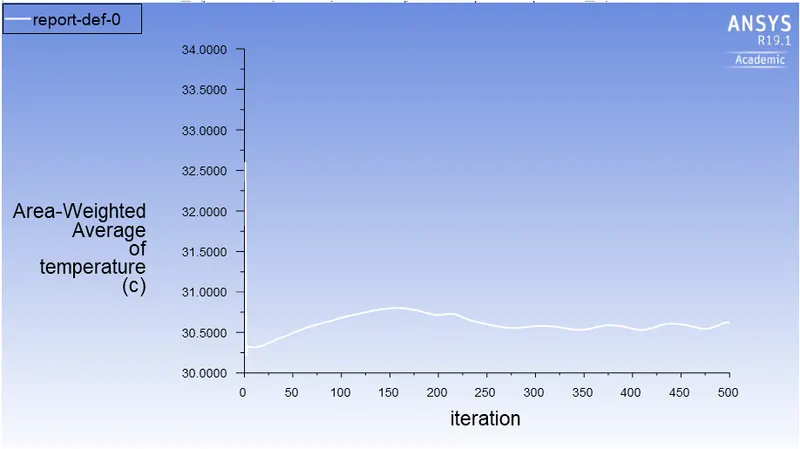
The results of k-omega SST model are as follows :

Residuals plot

Area weighted average plot for outlet temperature

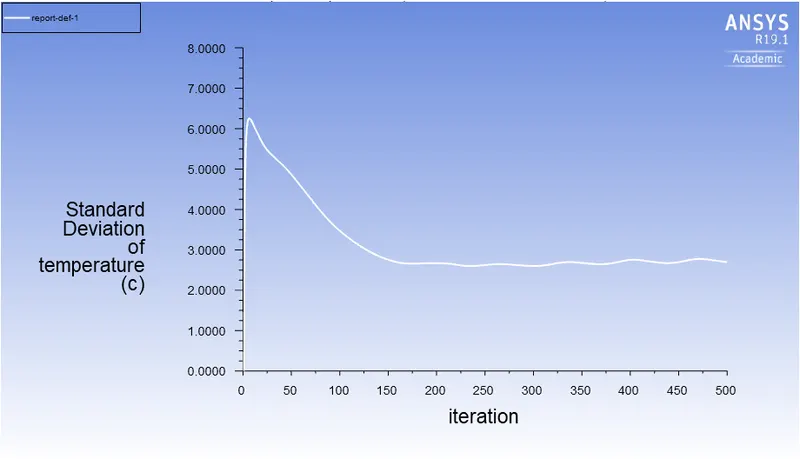
Standard deviation of temperature at the outlet

The results of k-epsilon SST model are as follows :

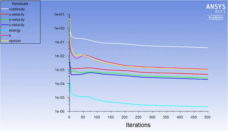
Residuals plot

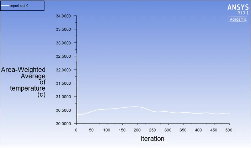
Area weighted average plot for outlet temperature

Standard deviation oftemperature at the outlet

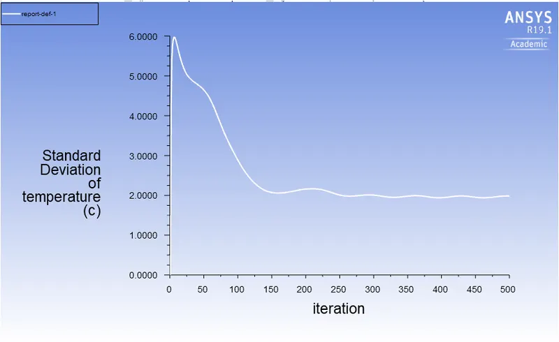
From the above results, it can be seen that standard deviation for k-Omega SST model is 2.697 whereas the standard deviation for k-epsilon model is 1.98. Since standard deviation for k-Omega SST model is more than standard deviation for k-epsilon model, it can be said k-epsilon method produces better simulation results than k-Omega SST model. Hence k-epsilon model is used for further simulation cases.

Temperature contour plots on the cut planes along and across the pipe.

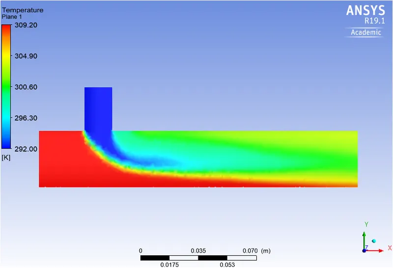
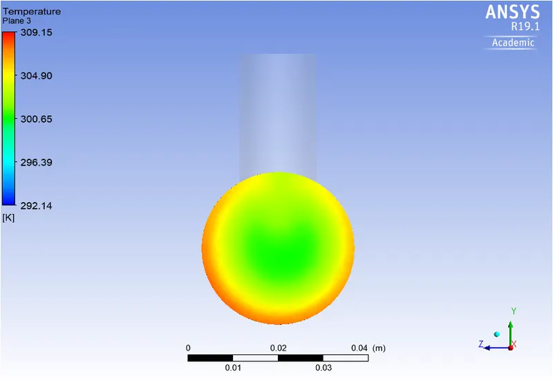
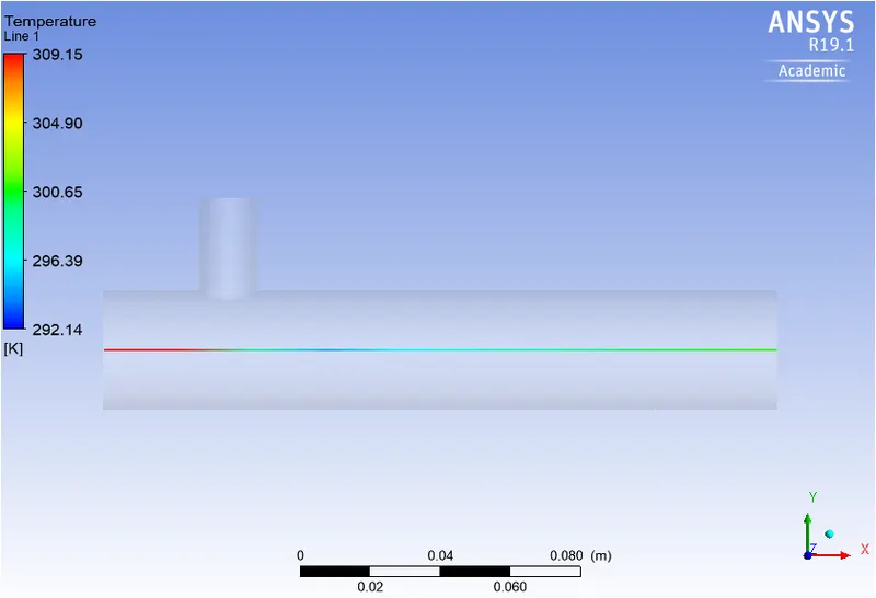
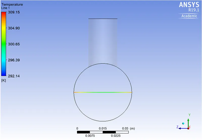
Temperature line plots along and across the length of the pipe

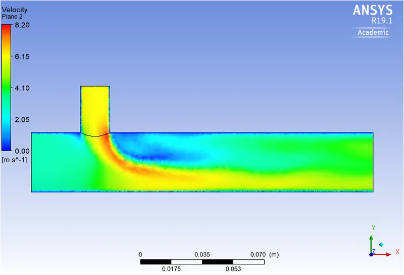
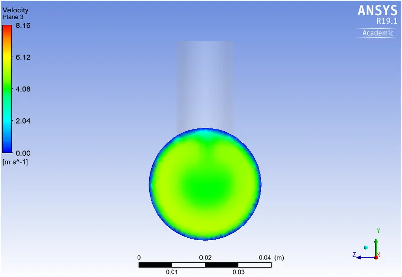
Velocity contour plots on the cut planes along and across the pipe.

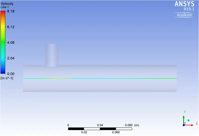
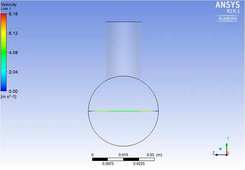
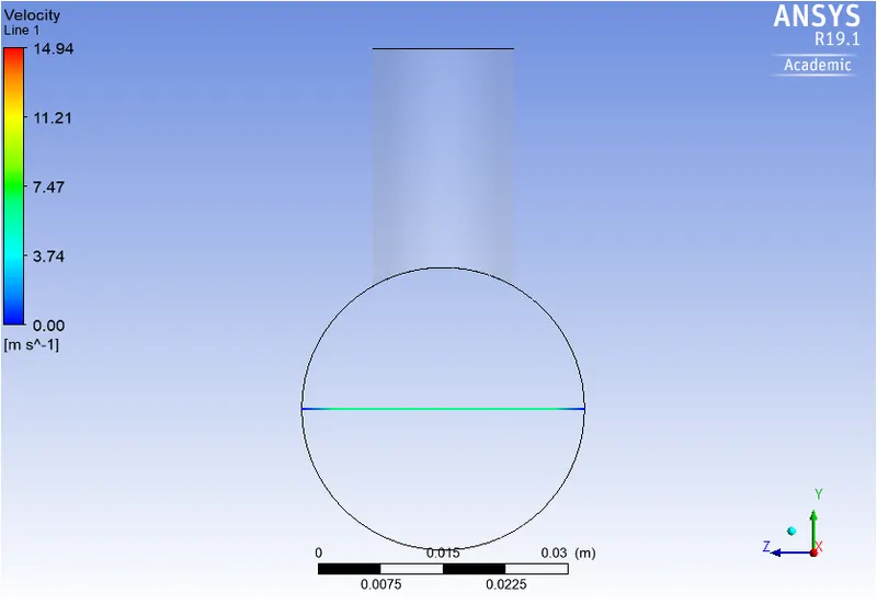
Velocity line plots along and across the length of the pipe

Case 2 : Short mixing tee with momentum ratio 4

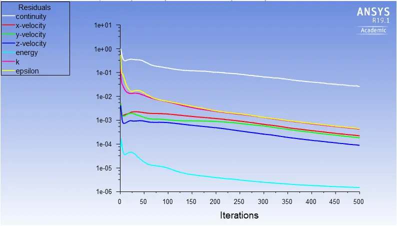
Residuals plot

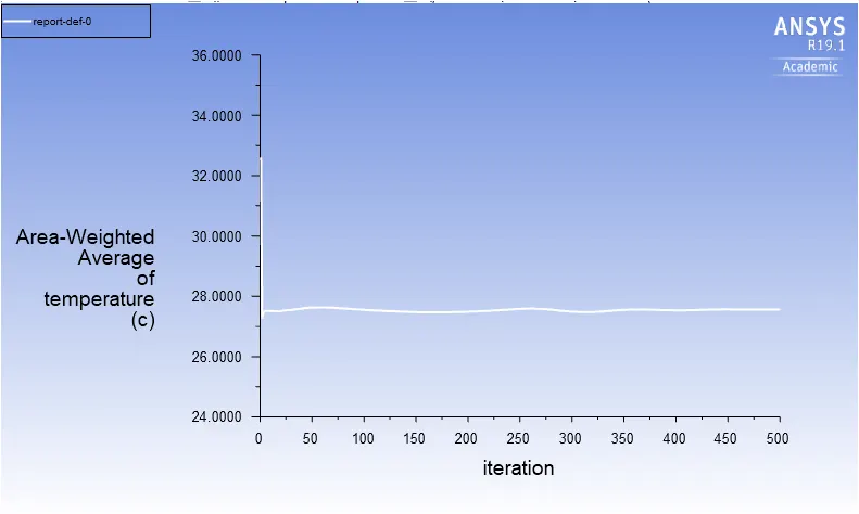
Area weighted average plot for outlet temperature

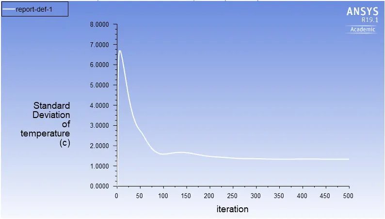
Standard deviation of temperature at the outlet

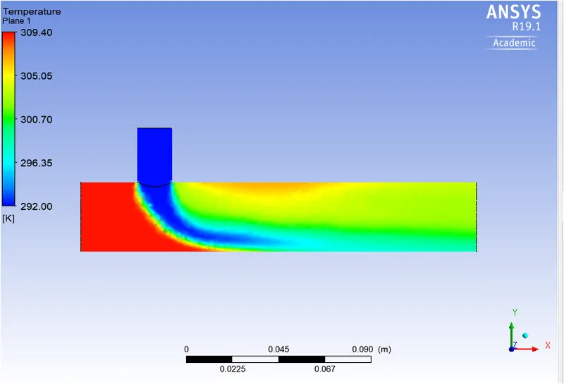
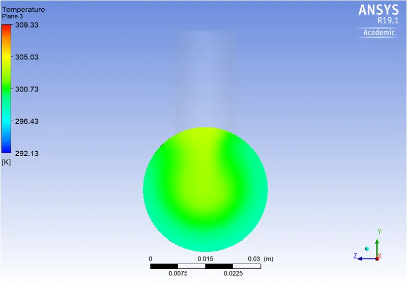
Temperature contour plots on the cut planes along and across the pipe.

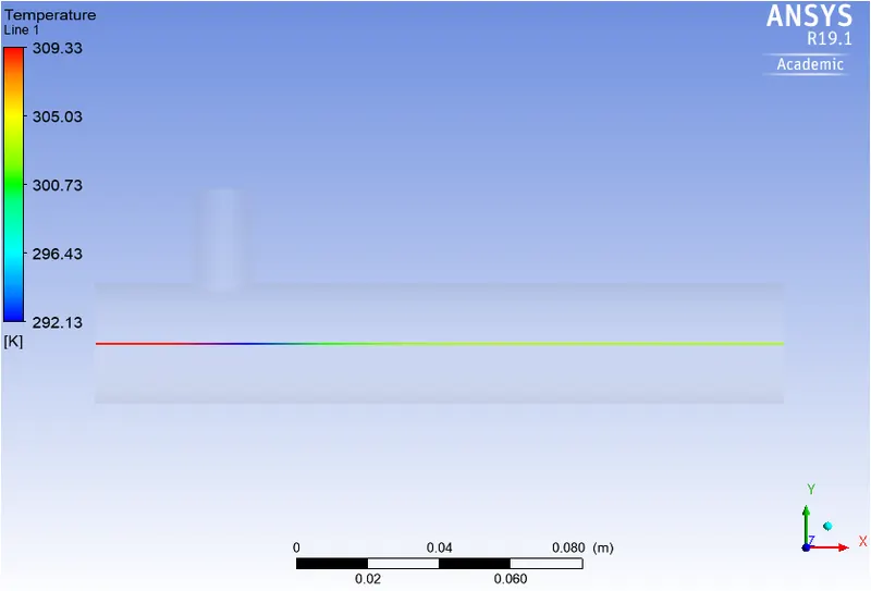
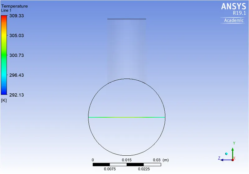
Temperature line plots along and across the length of the pipe

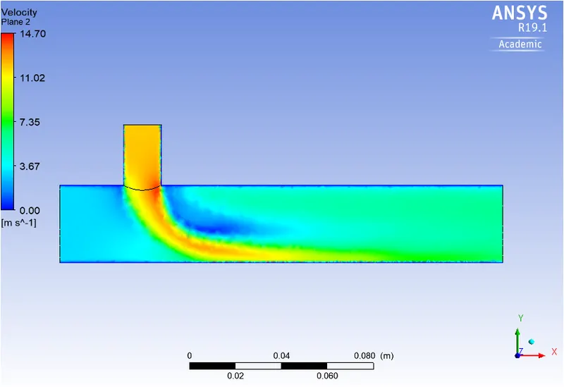
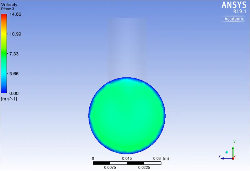
Velocity contour plots on the cut planes along and across the pipe.

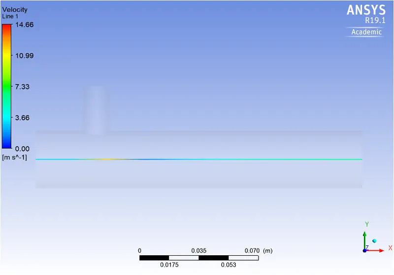
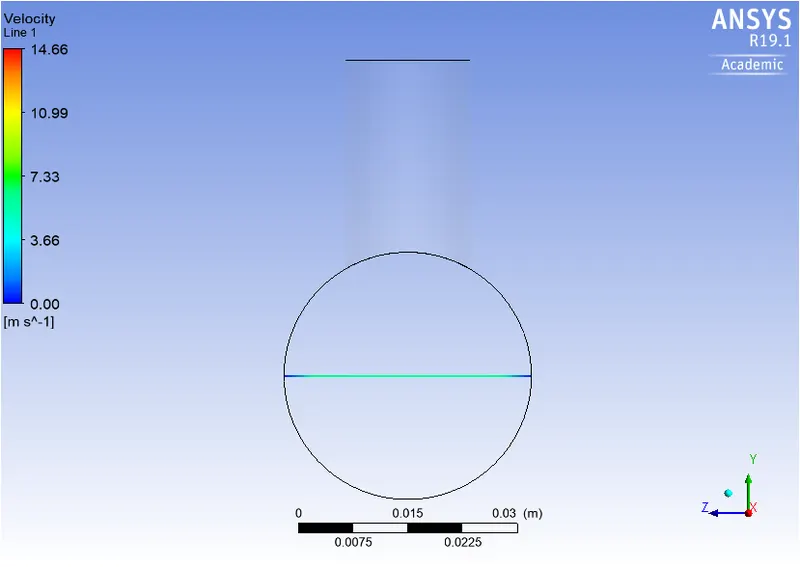
Velocity line plots along and across the length of the pipe

Case 3: Long mixing tee with momentum ratio 2

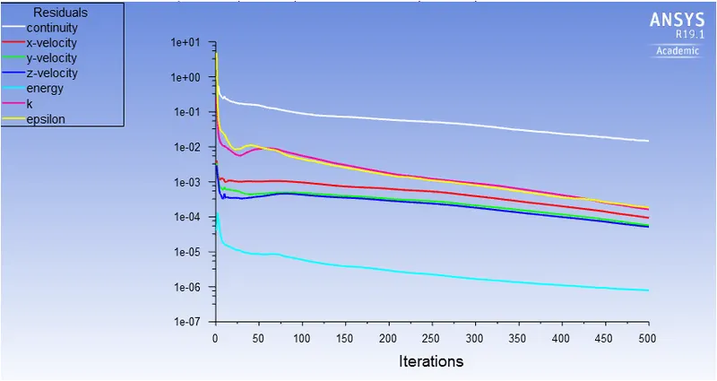
Residuals plot

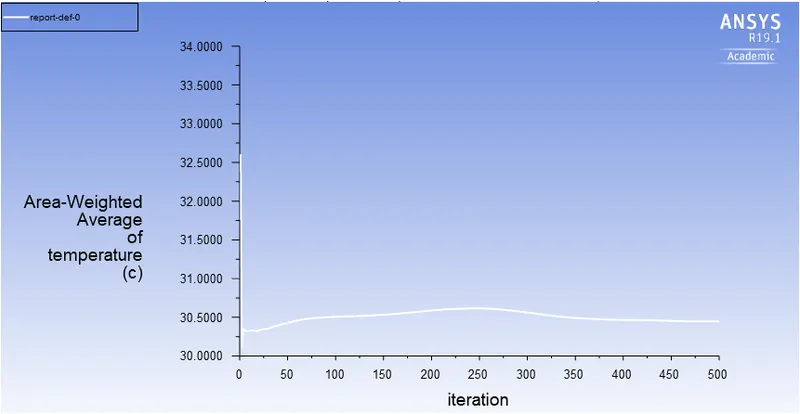
Area weighted average plot for outlet temperature

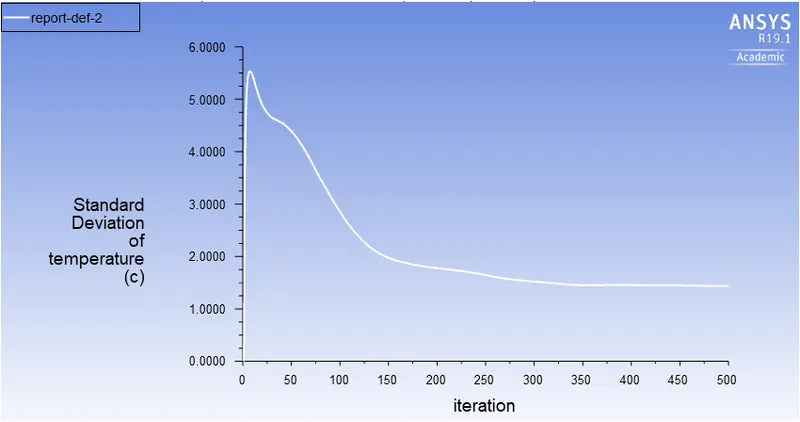
Standard deviation of temperature at the outlet

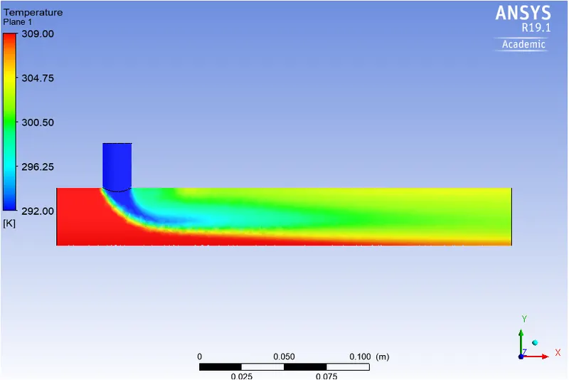
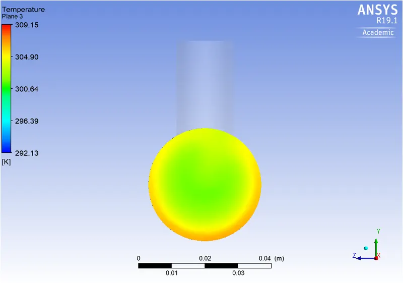
Temperature contour plots on the cut planes along and across the pipe.

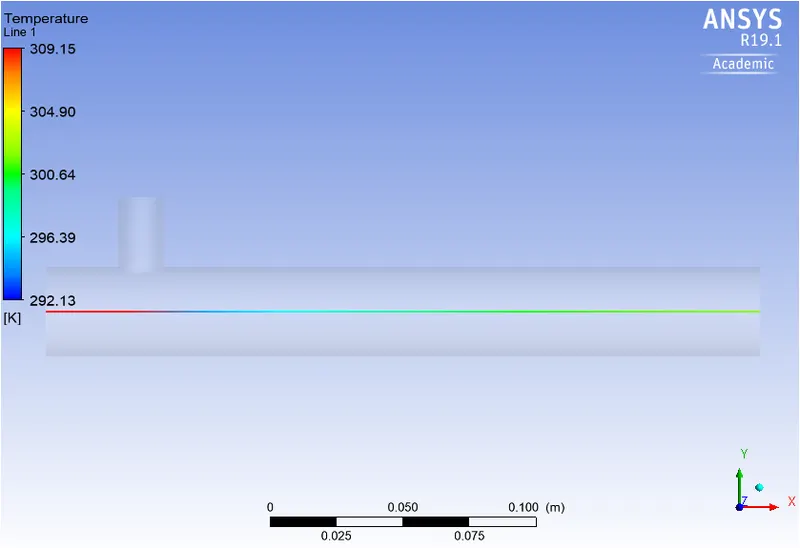
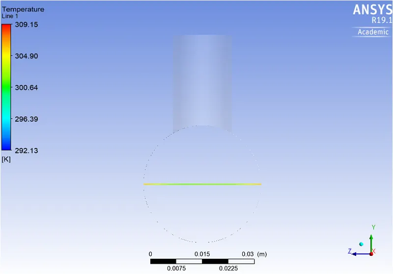
Temperature line plots along and across the length of the pipe

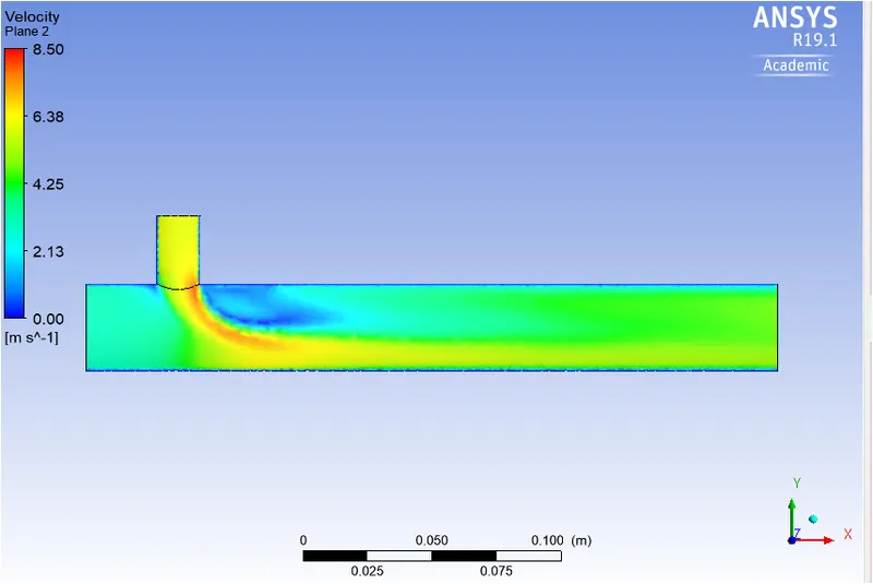
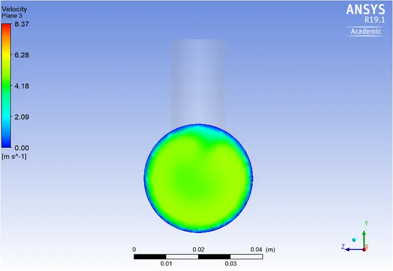
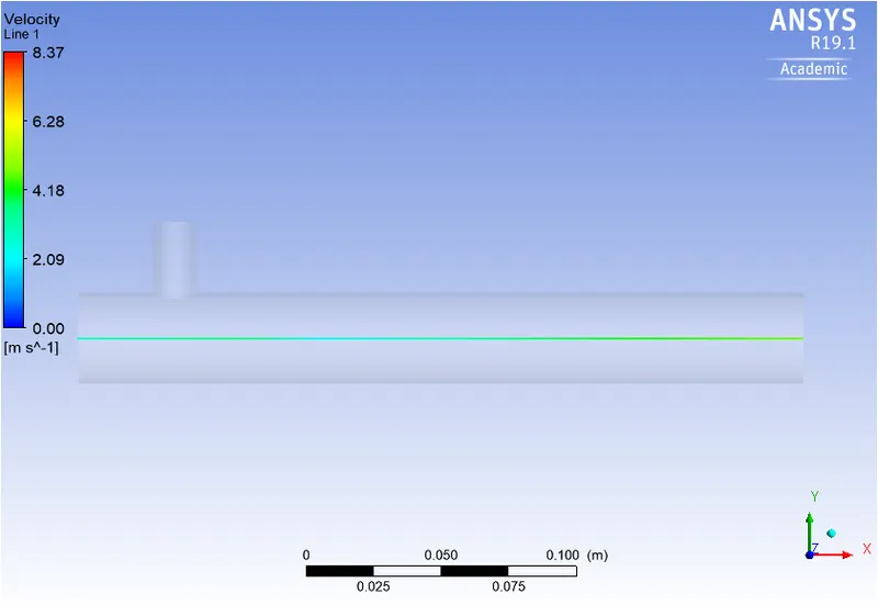
Velocity contour plots on the cut planes along and across the pipe.

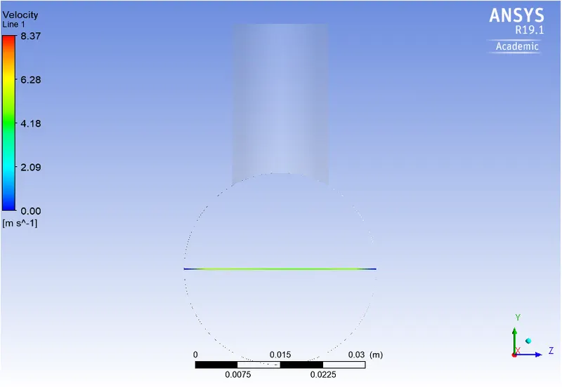
Velocity line plots along and across the length of the pipe

Case 4: Long mixing tee with momentum ratio 4

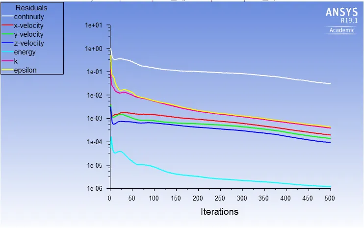
Residuals plot

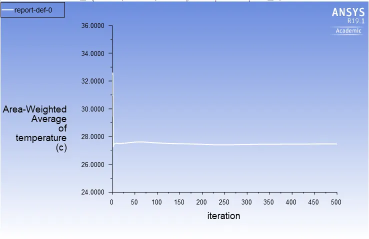
Area weighted average plot for outlet temperature

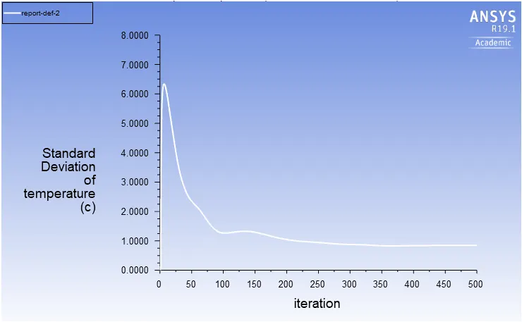
Standard deviation of temperature at the outlet

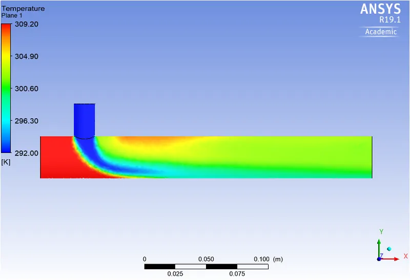
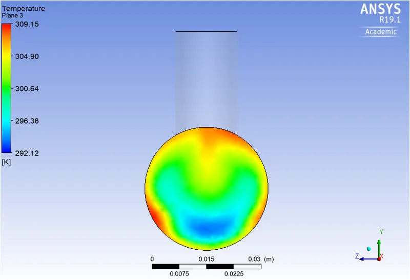
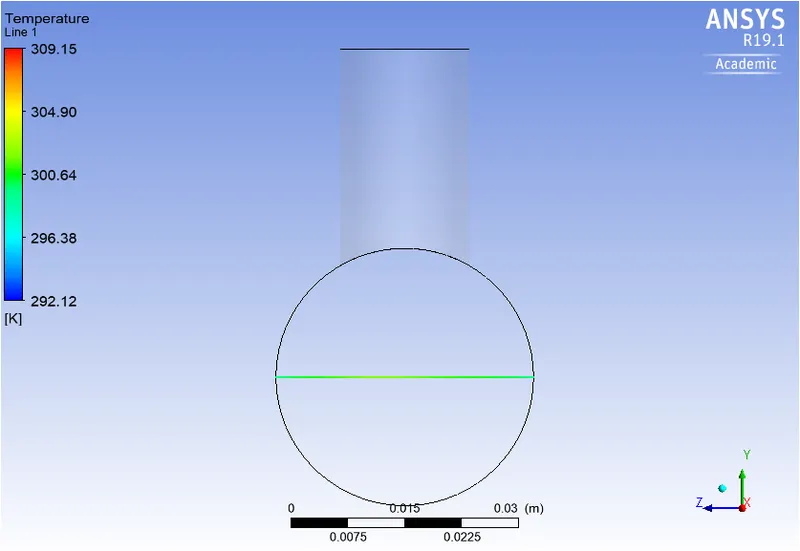
Temperature contour plots on the cut planes along and across the pipe.

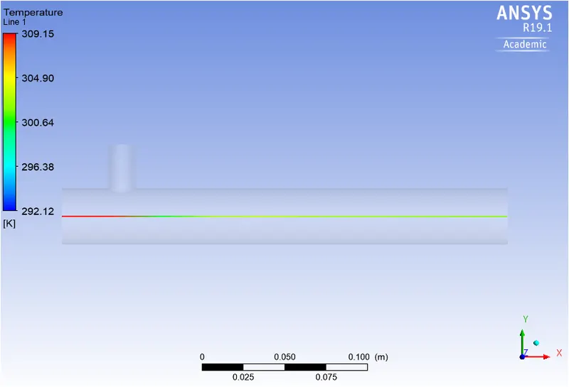
Temperature line plots along and across the length of the pipe

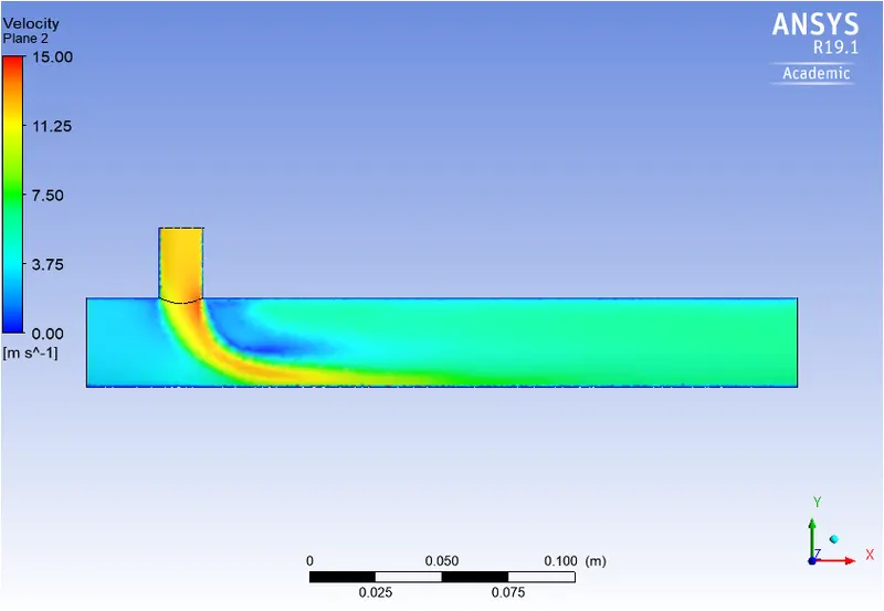
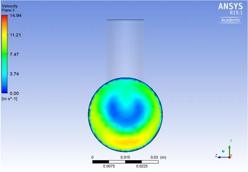
Velocity contour plots on the cut planes along and across the pipe.

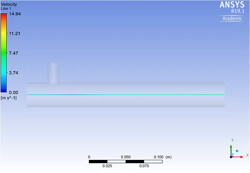
Velocity line plots along and across the length of the pipe

Comparison of different cases

Sr no	Case	Cell count	No of iterations required for convergence	Average outlet temperature (Kelvin)
1	Short mixing Tee with inlet velocity 3 m/s and momentum ratio 2	214218	150	303.53
2	Short mixing Tee with inlet velocity 3 m/s and momentum ratio 4	214218	200	300.71
3	Long mixing Tee with inlet velocity 3 m/s and momentum ratio 2	291675	200	303.59
4	Long mixing Tee with inlet velocity 3 m/s and momentum ratio 4	291675	250	300.62

Conclusion

The simulation was performed using k-omega SST model and k-epsilon model for selection of better model. The standard deviation for k-omega SST model was more which indicates that simulation results from this model would be less accurate. So k-epsilon model was used in performing this simulation.

The average temperature at outlet for both long and short tee are almost same for both the momentum ratios. Hence, it can be inferred that mixing efficiency is independent of length.

For both short and long tee, the average temperature at the outlet is lower for higher momentum ratio.

The standard deviation of temperature at the outlet is lower for higher momentum ratio. The simulated value of outlet temperature is closer to analytical value for higher momentum ratio. Thus mixing efficiency is better for higher momentum ratio.

Mesh independence study is important for any simulation as it helps to determine the appropriate mesh size which helps in decreasing computation power and cost required for the simulation.