Week 4 - CHT Analysis on Exhaust port

1. Description of why and where a CHT analysis is used.
2. Maintain the y+ value according to the turbulence model and justify the results.
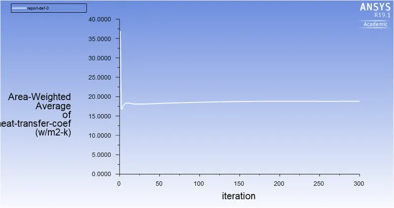
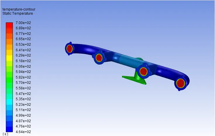
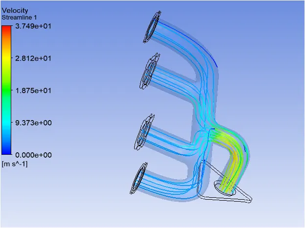
3. Calculating the wall/surface heat transfer coefficient on the internal solid surface & showing the velocity & temperature contours in appropriate areas.
4. How would HTC predictions from the simulations are verified and on what factors does the accuracy of the prediction depend on?

Conjugate Heat Transfer

The Conjugate Heat Transfer (CHT) analysis type allows for the simulation of heat transfer between solid and fluid domains by exchanging thermal energy at the interfaces between them. The conjugate procedure is an approach of determining the distribution of parmeters arising on the interface as a result of elements interaction. This is achieved by solving the governing equations for each interaction element and by following conjugation of these solutions at the interface.

Typical applications of conjugate heat transfer analysis are simulation of heat exchangers, cooling of electronic equipment, simulation of internal combustion engines, simulation of pumps and compressors and general-purpose cooling and heating systems.

Geometry

Loading of geometry in spaceclaim

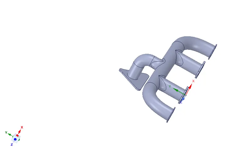
Check for any extra edges in the geomery and if there are any extra edges present, they are supposed to be removed.

Go to prepare-volume extract so as to separate fluid volume and solid volume. Move both the volume to new component and delete the empty components.

Share topology must be enabled for the geometry.

Next go to workbench-shareprep for achieving conformal mesh between fluid and solid domain. Pink circles would be visible after this process.

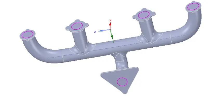
Creating Named Selections

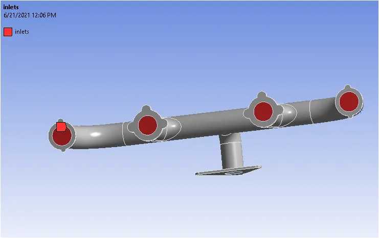
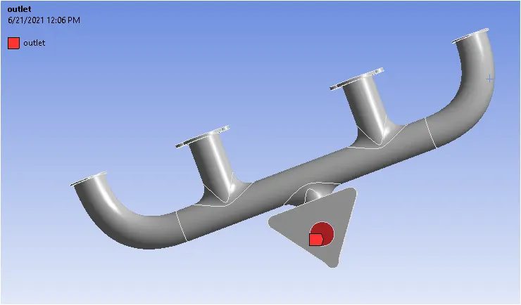
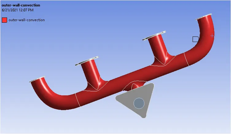
Ansys fluent names unmanes parts as wall and designates adiabatic boundary condition.

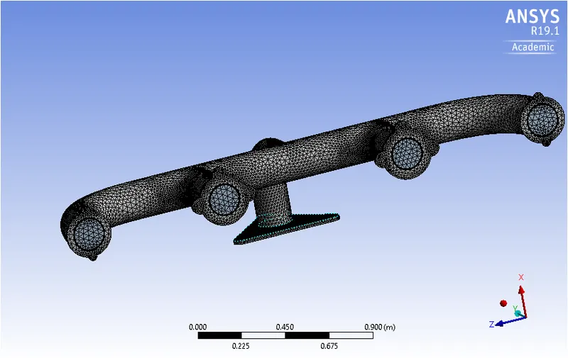
Initial mesh with element size of 0.15m is generated.

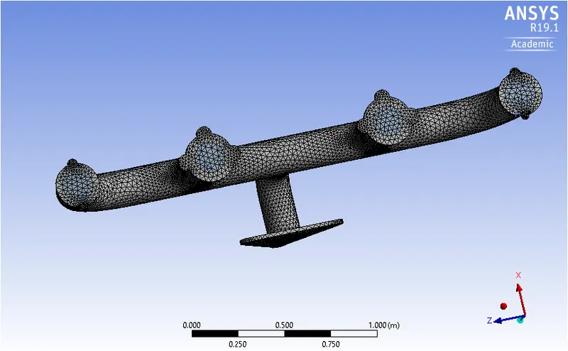
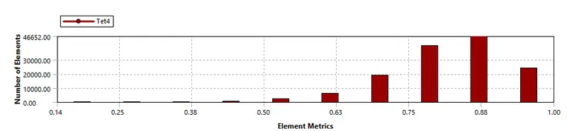
Mesh Quality

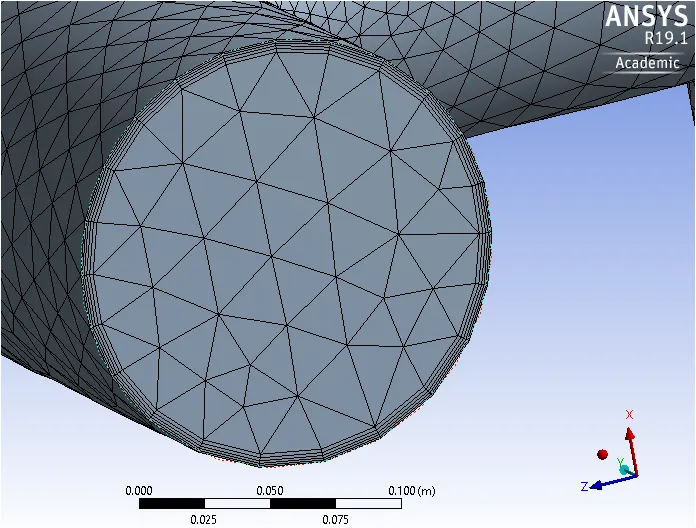
Now hiding the outer body and generating inflation layers for inner body.

Refining the mesh of outer body by reducing the element size to 0.01m

Setting up physics

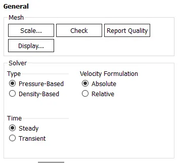
Solver

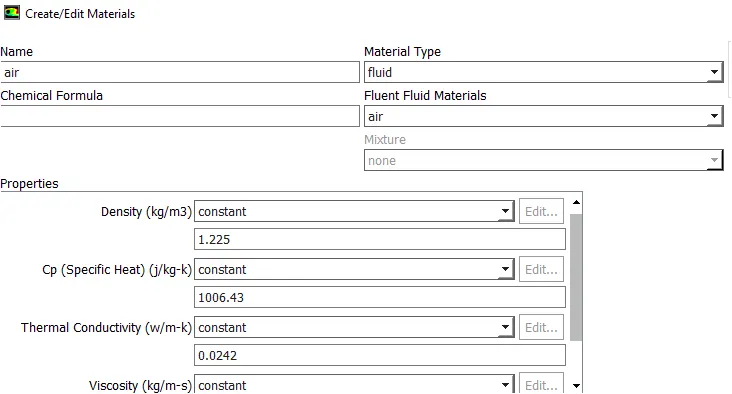
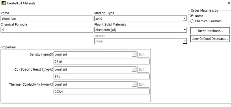
Material Selection

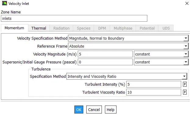
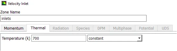
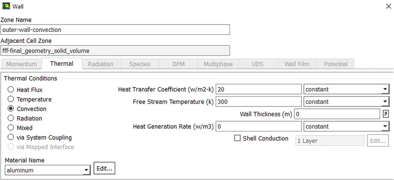
Boundary Conditions

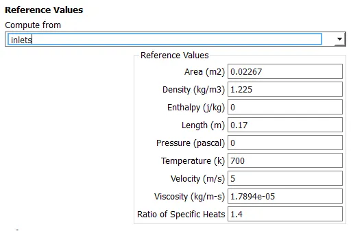
Reference Values

Post Processing and results

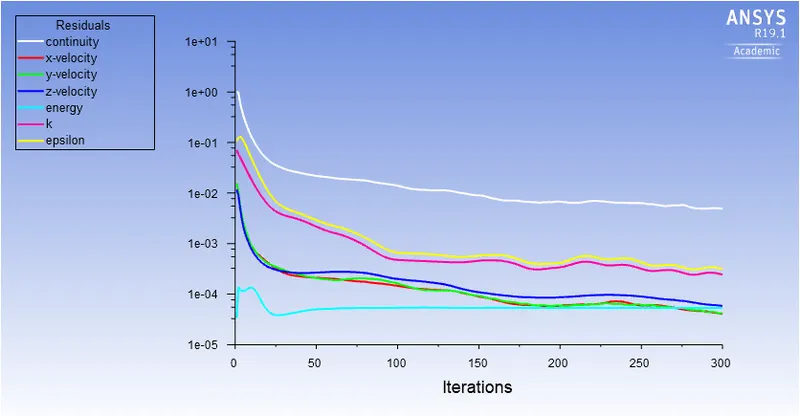
Case 1

Inner body mesh size - 0.15m

Outer body mesh size - 0.15m

No inflation layers

K-epsilon method

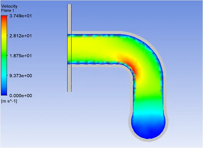
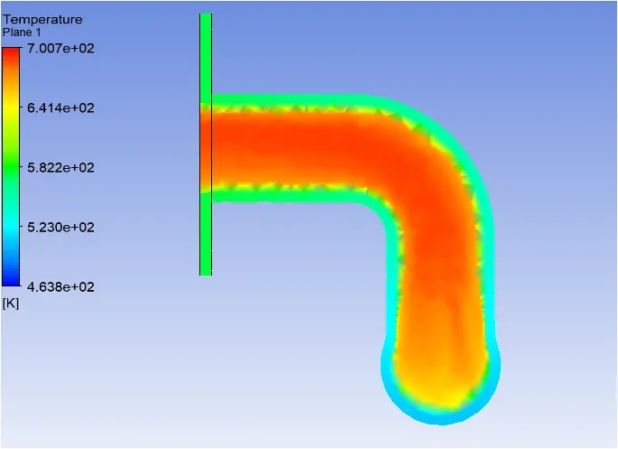
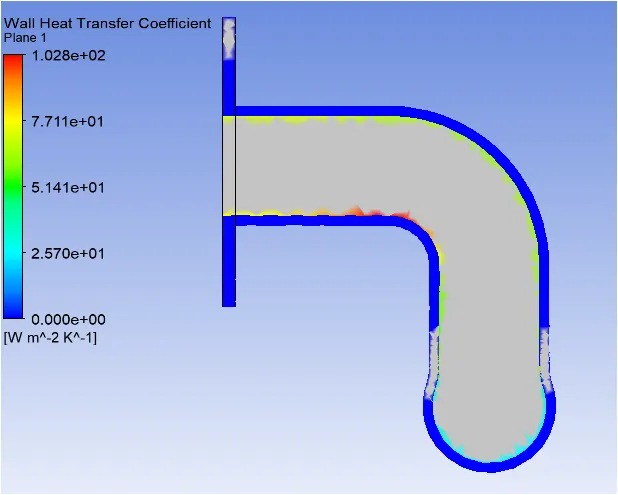
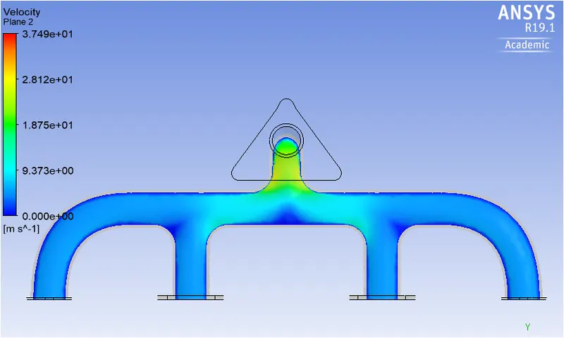
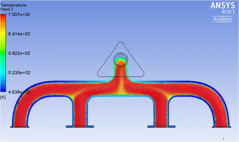
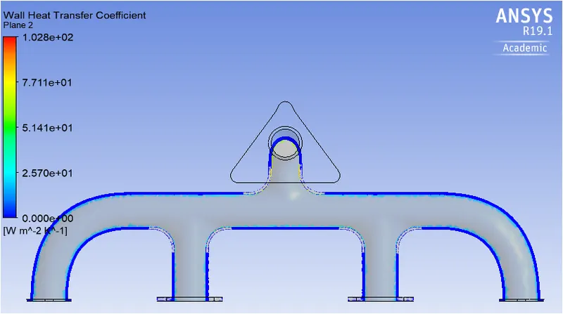
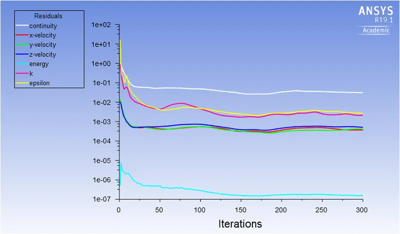
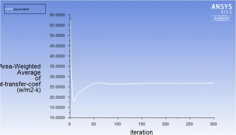
Case 2

Inner body mesh size - 0.15m

Outer body mesh size - 0.01m

K-epsilon method

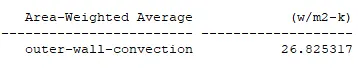
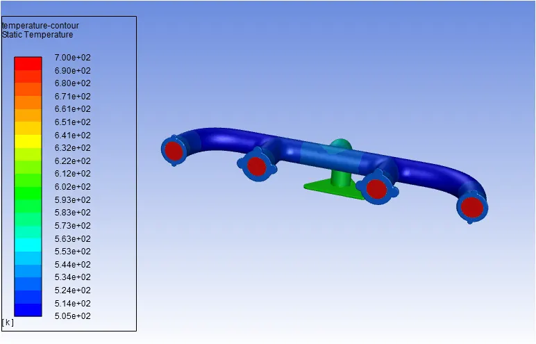
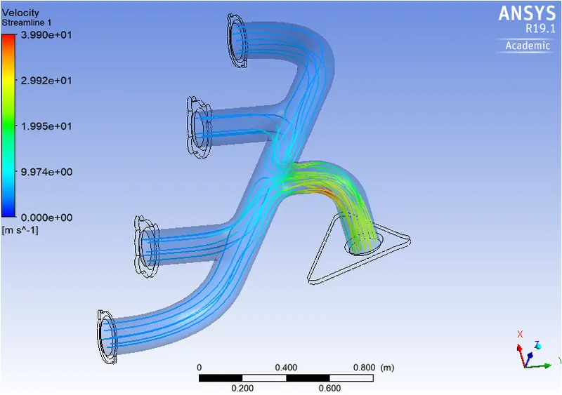
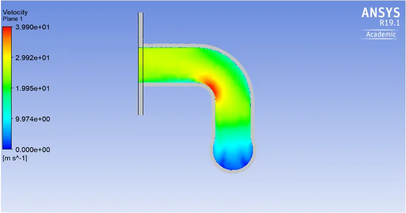
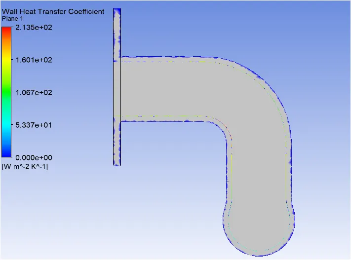
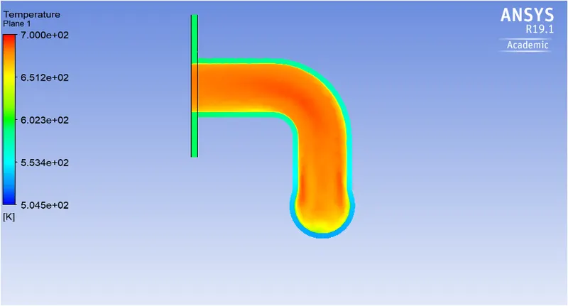
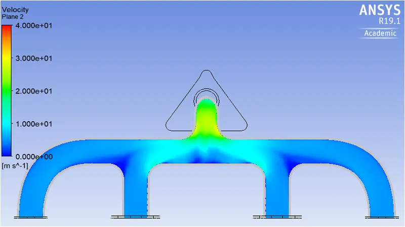
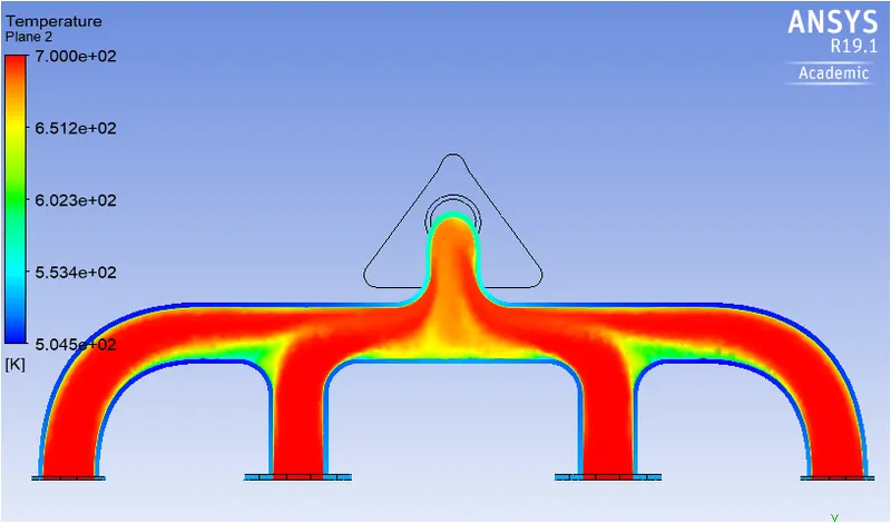
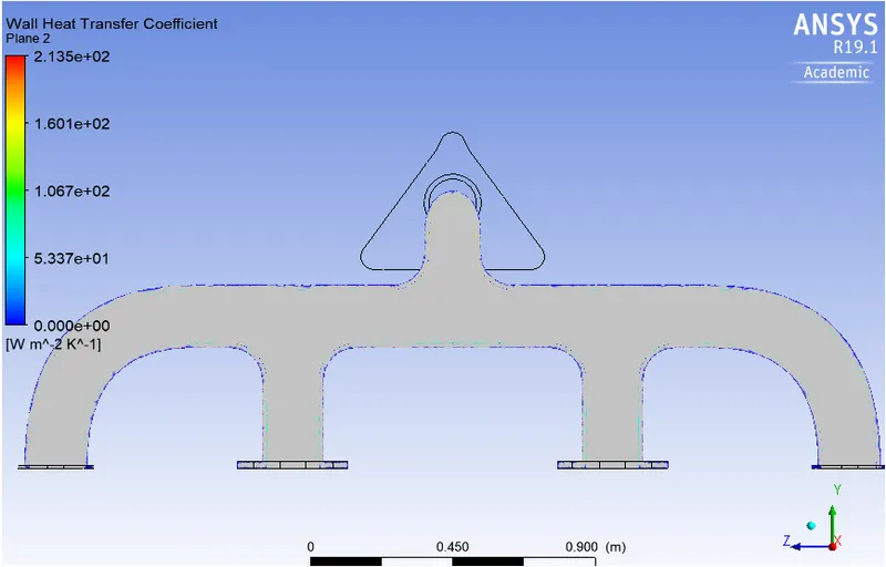
Case 3

Inner body mesh size - 0.15m

Outer body mesh size - 0.01m

K-Omega method

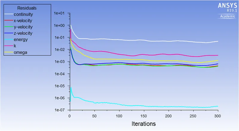
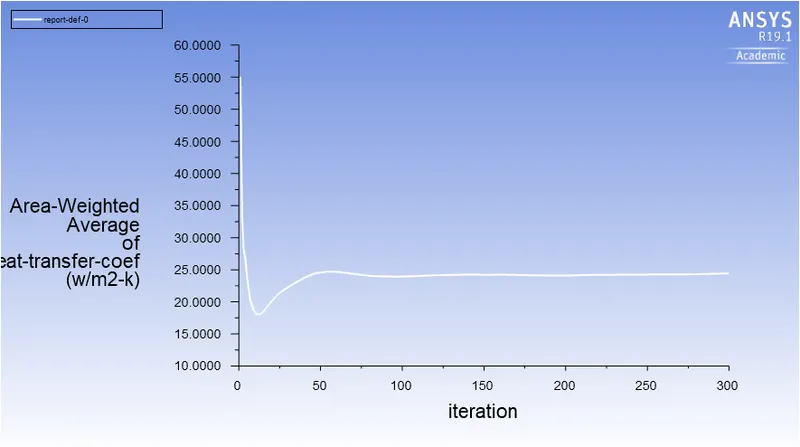
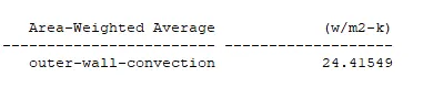
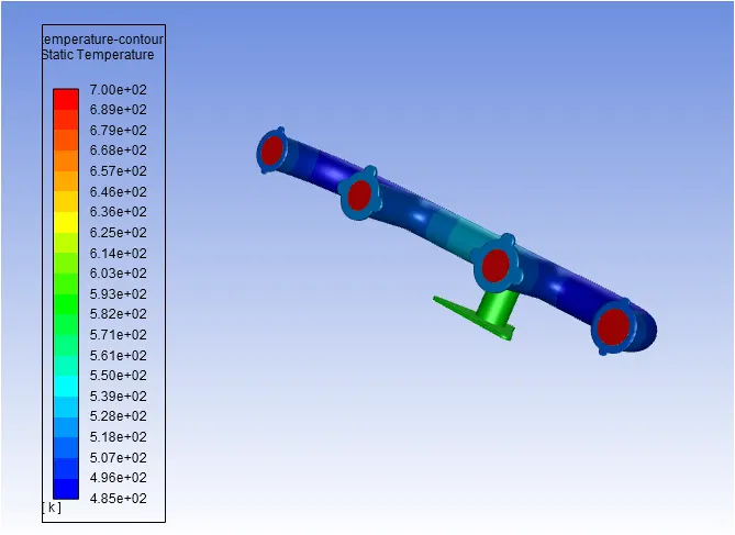
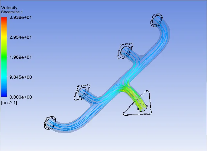
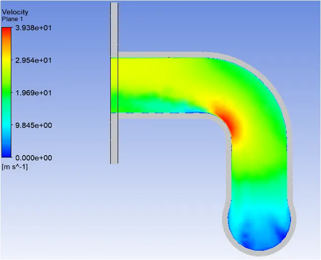
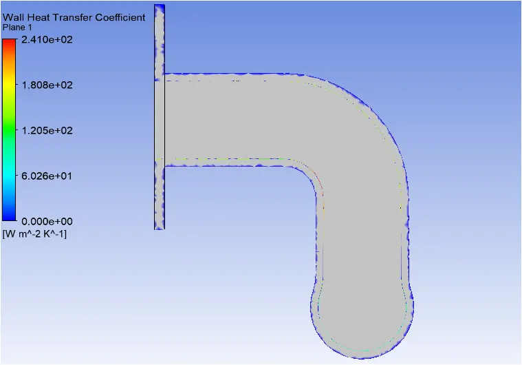
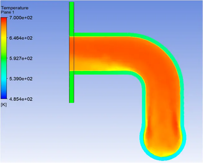
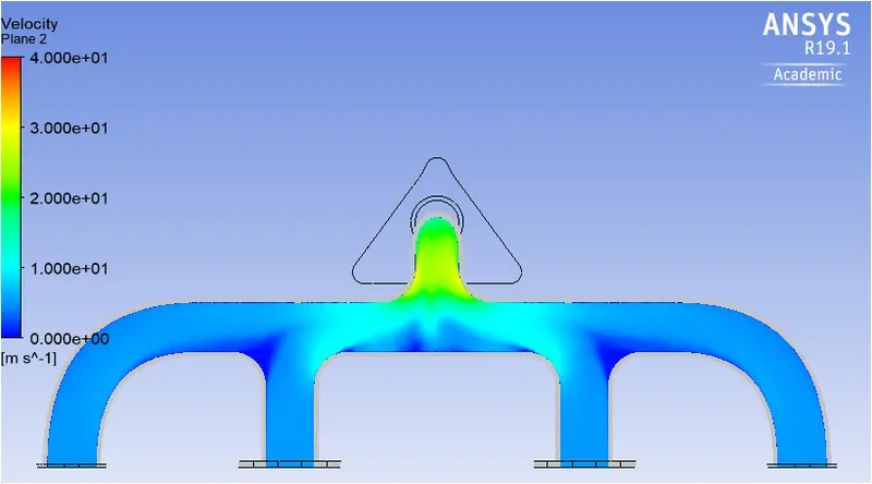
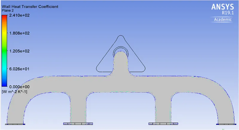
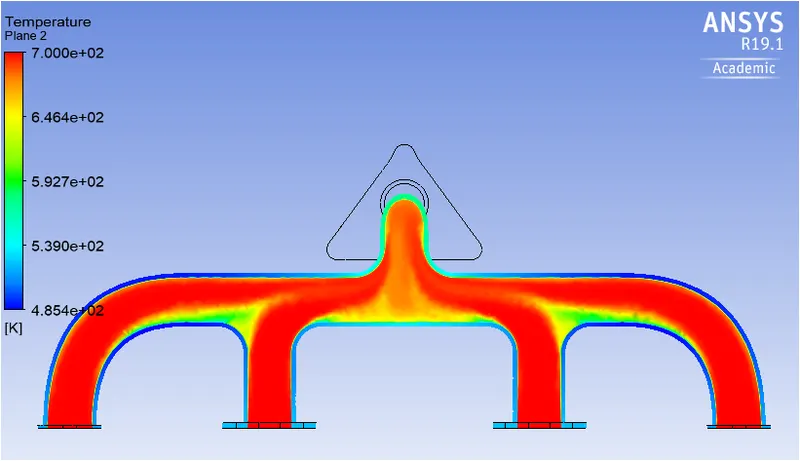
Wall heat transfer coefficient for different conditions

Sr No	Viscous Model	Number of mesh elements	Wall heat transfer coefficient (W/m2K)
1	K-epsilon	138036	18.783
2	K-epsilon	478144	26.825
3	K-Omega	478144	24.415

Verification of HTC

Using the properties of air, the Reynolds number for the flow considered flow is 58189.89 . Hence, the nature of flow is turbulent.

Analytically, Dittus Boelter equation can be used to determine the heat transfer coefficient. Dittus Boelter equation is as follows :

Nu = 0.023*Re^0.8*Pr^0.4

Where Re = ρVD/μ

Pr = μCp/K

Nu = hL/K

Using the above co-relations, the value of heat transfer coefficient h can be determined. Although all the conditions of Dittus Boelter equation are not satisfied but most of the conditions are met and hence can be used for validation purpose.

Factors affecting quality of prediction

Use of refined mesh and appropriate Y+ leads to better results of simulation.

Selection of appropriate solver and turbulence method.

Selection of proper boundary conditions.

Conclusion

From the above simulation, it can be said that the results for all the cases are almost same but appropriate selection of mesh refinement and y+ selection gives more accurate results.

The velocity of flow is maximum at the oulet. This is due to the conservation of momentum as exhaust valve has 4 inlets and only one outlet.

The maximum heat transfer coefficient occurs at the bend prior to the outlet. This is because the velocity is higher at the outlet which increases the Reynolds number. With increase in Reynolds number, Nusselt number also increases due to which heat transfer coefficient also increases.