Week 2 - Flow over a Cylinder.
AIM:
To simulate the flow over a cylinder and explain the phenomenon of Karman vortex street.
OBJECTIVE:
- Simulate the flow with the steady and unsteady case and calculate the Strouhal Number for Re= 100.
- Calculate the coefficient of drag and lift over a cylinder by setting the Reynolds number to 10,100,1000,10000 & 100000. (Run with steady solver)
- Discuss the effect of Reynolds number on the coefficient of drag.
Vortex shedding.
In fluid dynamics, vortex shedding is an oscillating flow that takes place when a fluid such as air or water flows past a bluff (as opposed to streamlined) body at certain velocities, depending on the size and shape of the body. In this flow, vortices are created at the back of the body and detach periodically from either side of the body forming a Von Karman vortex street. The fluid flow past the object creates alternating low-pressure vortices on the downstream side of the object. The object will tend to move toward the low-pressure zone.
If the bluff structure is not mounted rigidly and the frequency of vortex shedding matches the resonance frequency of the structure, then the structure can begin to resonate, vibrating with harmonic oscillations driven by the energy of the flow. This vibration is the cause for overhead power line wires humming in the wind, and for the fluttering of automobile whip radio antennas at some speeds. Tall chimneys constructed of thin-walled steel tubes can be sufficiently flexible that, in air flow with a speed in the critical range, vortex shedding can drive the chimney into violent oscillations that can damage or destroy the chimney.
In the below gif we can observe the vortex shedding.
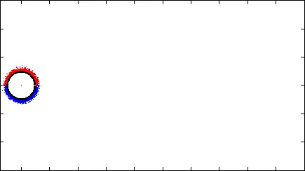
Karman vortex street.
A vortex street will form only at a certain range of flow velocities, specified by a range of Reynolds number(Re), typically above a limiting Re value of about 90. The (global) Reynolds number for a flow is a measure of the ratio of inertial to viscous forces in the flow of a fluid around a body or in a channel and may be defined as a nondimensional parameter of the global speed of the whole fluid flow.
Strouhal number.
The Strouhal number is a dimensionless number describing oscillating flow mechanisms,
The Strouhal number is often given as,
St=fL/V.
where f is the frequency of vortex shedding
L is the characteristic length
U is the flow velocity
PROCEDURE.
- Drag and drop the fluid flow fluent file from the tool box.
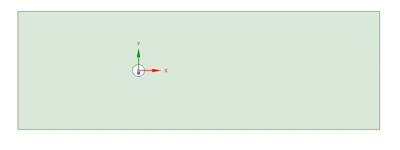
- Get into the geometry by double click and then create the geometry as required we have created the geometry which is shown in the figure for the flow over cylinder.
GEOMETRY.
- Then close the geometry and go to the mesh and make the required refinement for the mesh and here I have taken the element size as 0.15m and then in the sizing go to type then select number of divisions enter 36 then generate mesh and then go to inflation select face on which we are interested the inflation option helps to create body fitted mesh and then go to named selection and enter the boundary name and update the mesh and exit.
MESH.
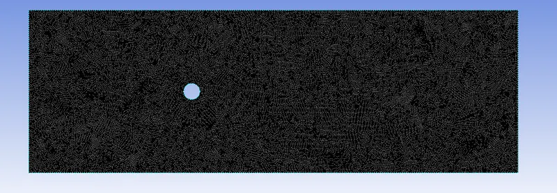
CELL COUNT.
Element size: 0.15m
Nodes: 56436
Elements: 111512
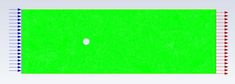
left side which is labelled with the blue arrows is the inlet and the one which is shown with the red arrows is the outlet and the top and bottom are symmetry boundaries.
- Then go to the setup >physics>viscous>laminar and also go to solution>select steady and pressure based solver
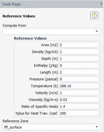
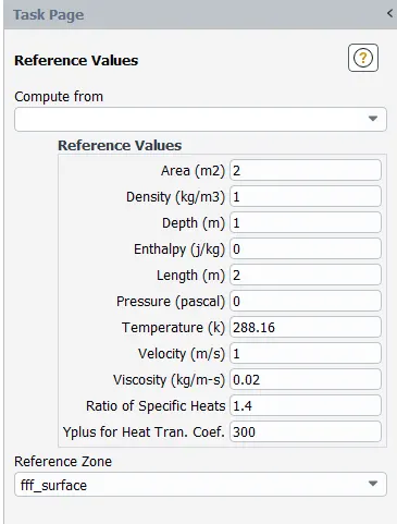
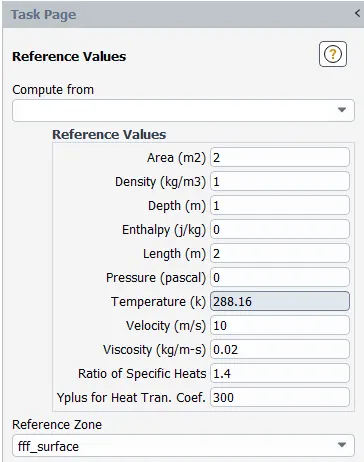
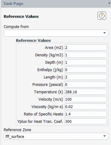
- and again go to physics>fluent database > select air and copy >ok then go to fluent fluid materials>select unwanted materials and delete. Before this go to zones>cell zones>set to user material>ok and then only we can delete the air option also in the materials and again go to materials > properties>density set it as 1 and viscosity as 0.02 then click on change/create.
- Then go to physics>boundaries>set the inlet velocity and check the outlet gauge pressure and the cylinder wall as noslip condition and also the symmetry boundary condition.
- And then go to post processing >surface>create >point (create a point at some distance from the cylinder so that we can observe the velocity at that point and then go to solution>Definition>New>Surface Report>Vortex Average>set variable as velocity > velocity magnitude and name the graph as monitor point velocity and check for the report plot and report file then apply and close.
- Then solution>initialization>method>hybrid and go to activities there give auto save and then initialize and then enter the number of iteration and then run the calculation.
- And as the simulation get over go to solution and get the plots and reports and in the results we can observe the contour plane and the animation can be obtained of our simulation.
RESULTS.
CASE 1.
Reynolds Number: 100
Steady flow simulation.
Viscosity: 0.02
Density of the fluid:1 kg/m^3
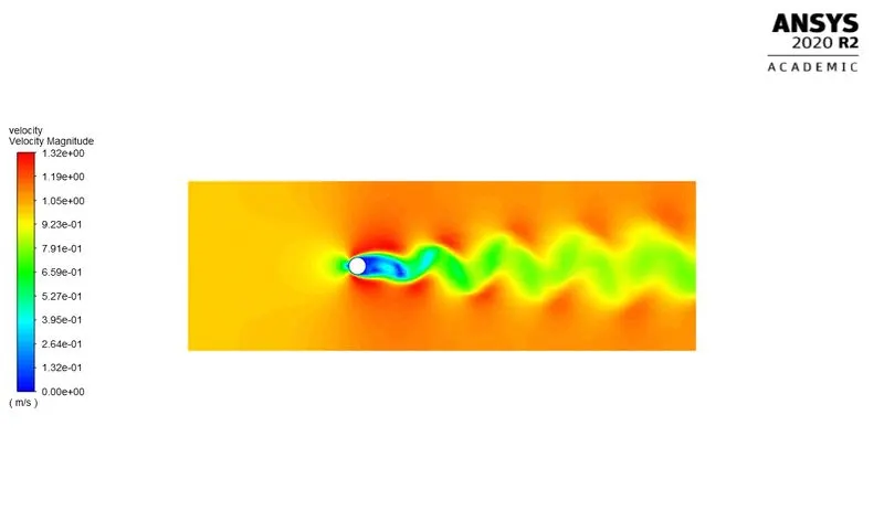
The velocity contour plane.
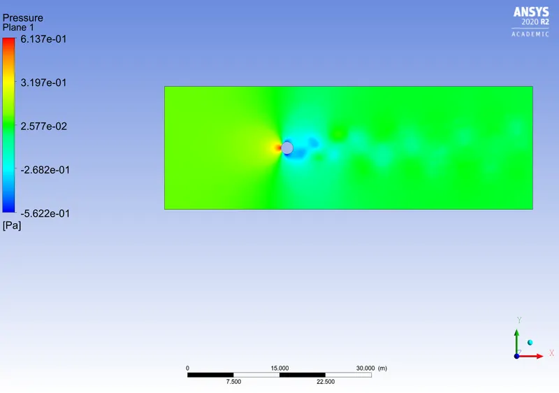
Pressure contour.
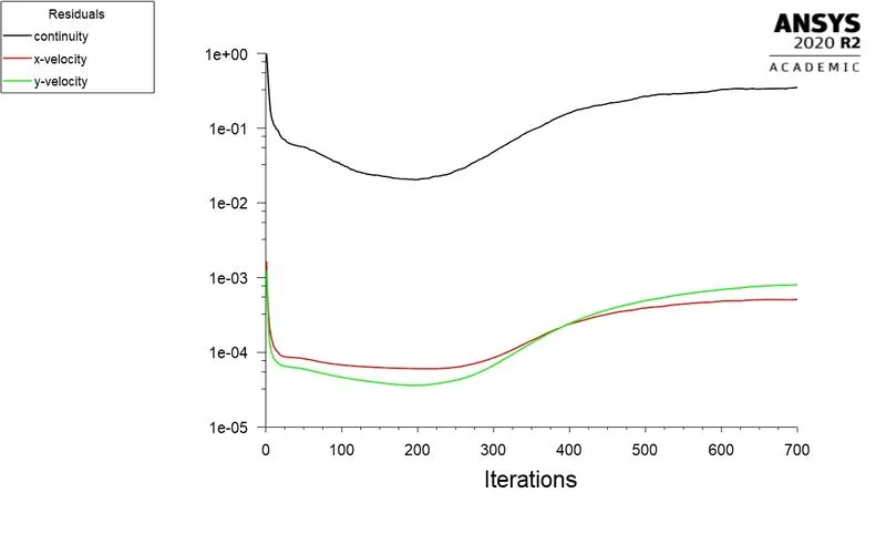
Residuals plot for Re 100 for the steady flow.
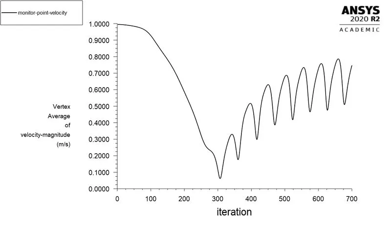
Monitor point velocity for Re 100 for the steady flow.
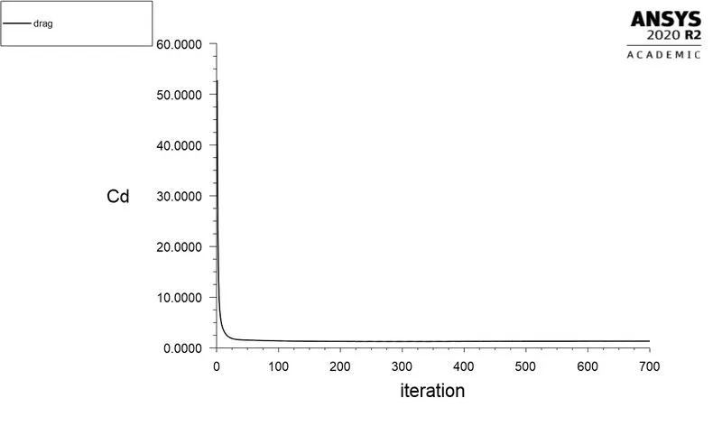
Drag coefficient.
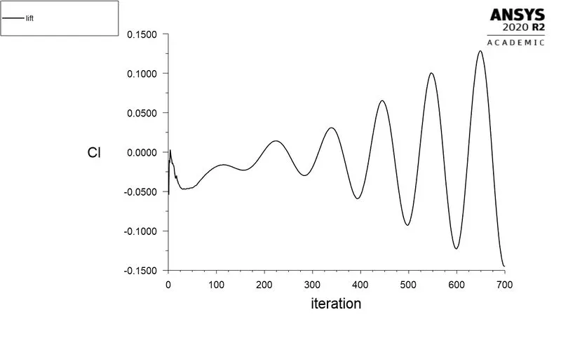
Lift coefficient.
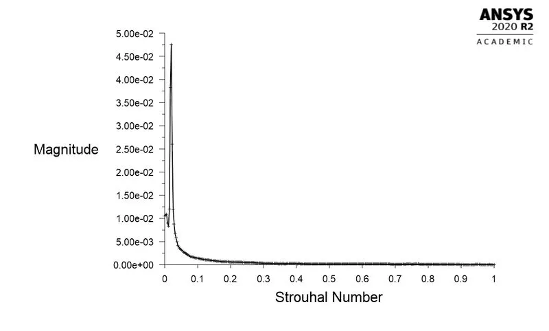
Spectral analysis of lift coefficient.
CASE 2.
Reynolds Number: 100
Transient flow simulation.
Viscosity: 0.02
Density of the fluid:1 kg/m^3
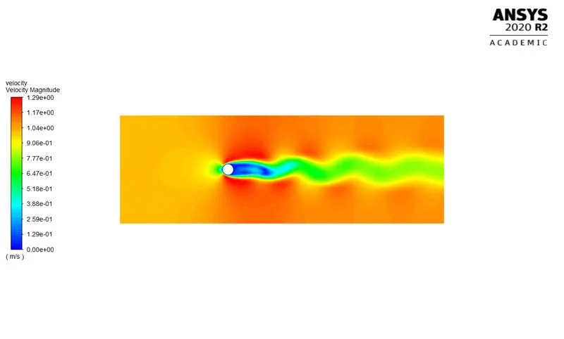
Velocity contour for Re 100 for the transient flow simulation.
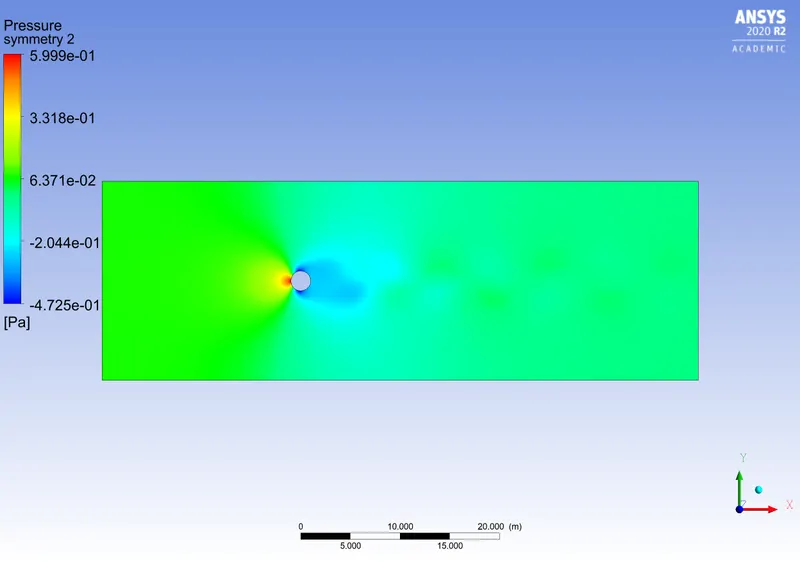
Pressure contour for Re 100 for transient flow.
Animation created for transient flow simulation.
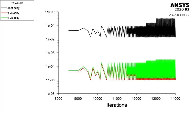
Residuals plot for Transient flow with Re 100. We can observe that how the solution is converging in the plot.
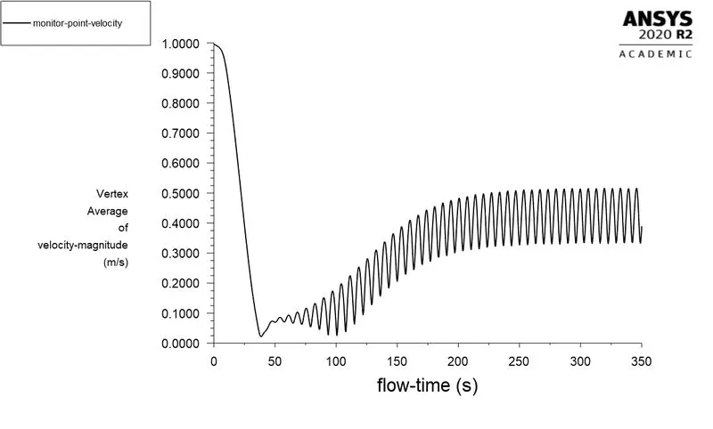
Monitor point velocity for Transient flow for Re 100. We can observe that how the solution is converging in the plot.
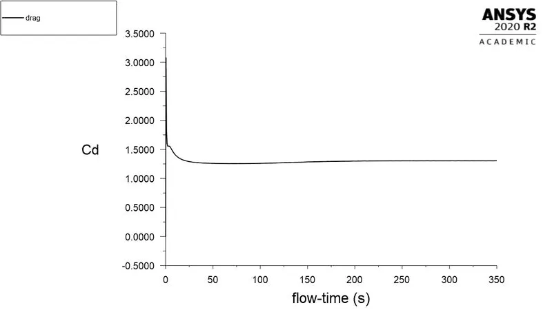
Drag coefficient.
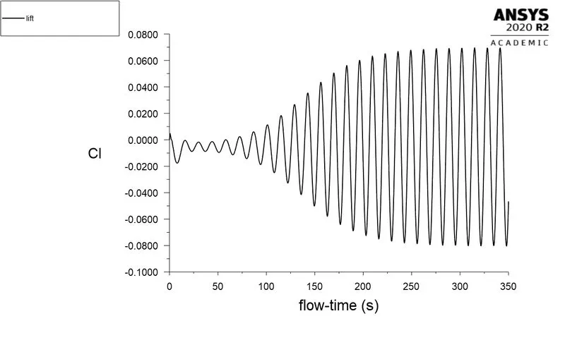
Lift coefficient.
Spectral analysis of lift coefficient.
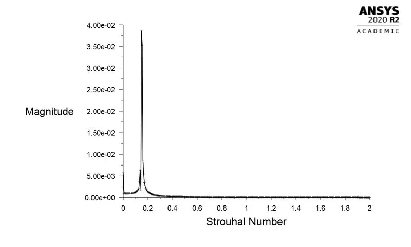
Equation used to calculate the Strouhal Number.
Strouhal Number=`(f*L)/U`
where,
f is the frequency
L is the characteristic length
U is the velocity
| Reynolds Number | Solver | Cd | Cl | Velocity at the monitor point(m/s) | strouhal Number |
| 100 | Steady flow | 1.3439732 | -0.12644603 | 0.57676452 | 1 |
| 100 | Transient flow | 1.3045044 | -0.04661765 | 0.38936356 | 1.997147 |
CASE 3.
Reynolds Number: 10
Steady flow simulation.
Viscosity: 0.02
Density of the fluid:1 kg/m^3
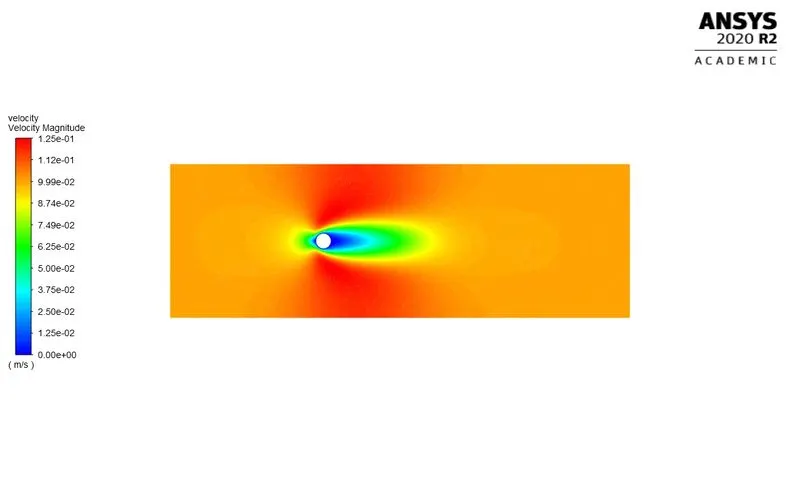
Velocity contour for Re 10.
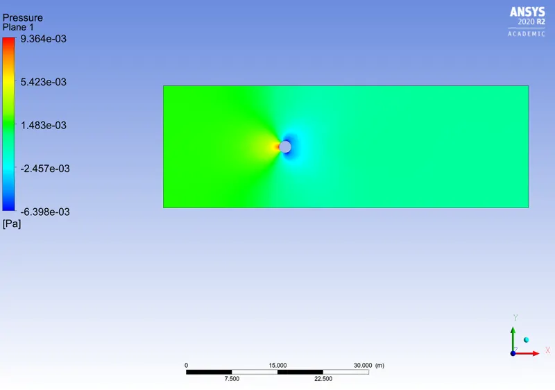
Pressure contour for Re 10.
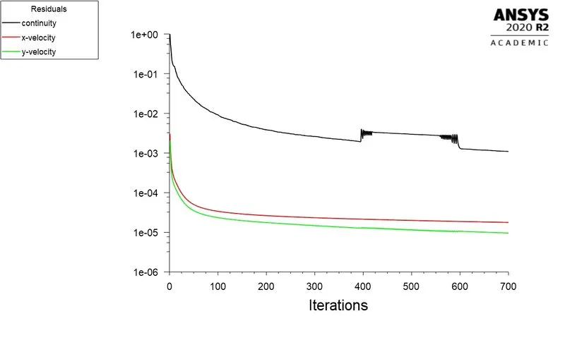
Residuals plot.
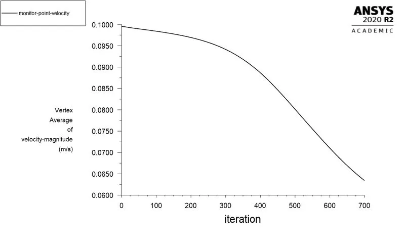
Monitor point velocity.
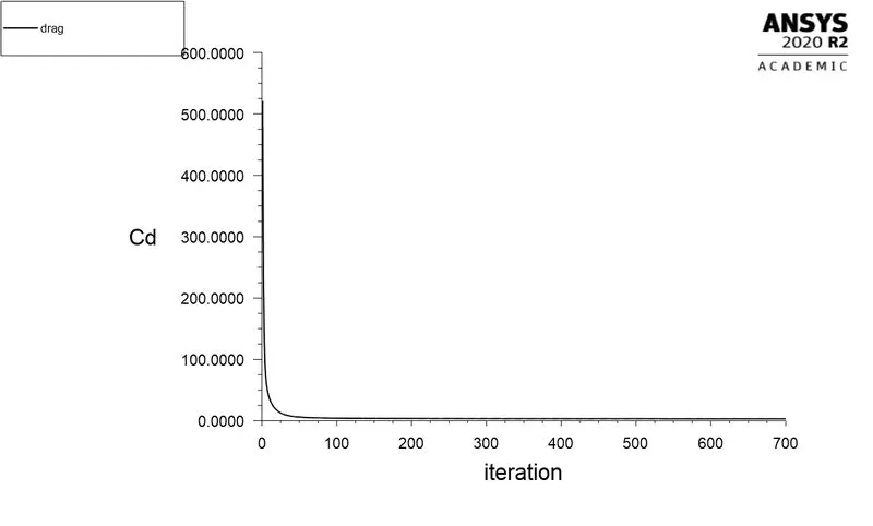
Drag coefficient.
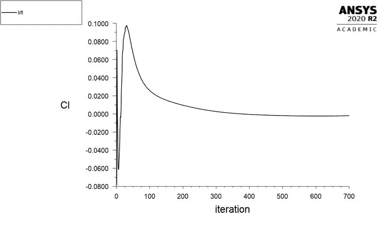
Lift coefficient.
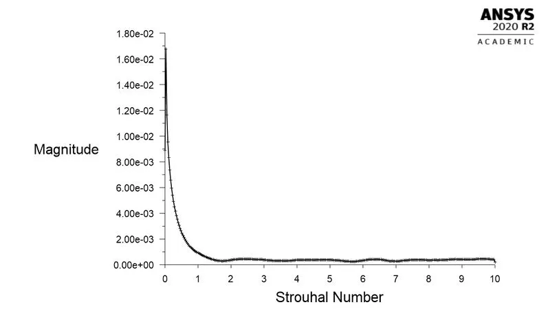
Spectral analysis of lift coefficient.
CASE 4.
Reynolds Number: 1000
Steady flow simulation.
Viscosity: 0.02
Density of the fluid:1 kg/m^3
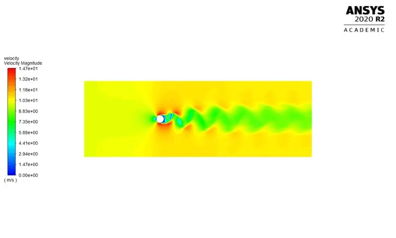
Velocity contour.
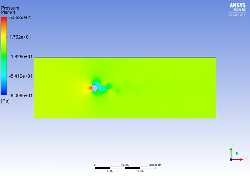
Pressure contour.
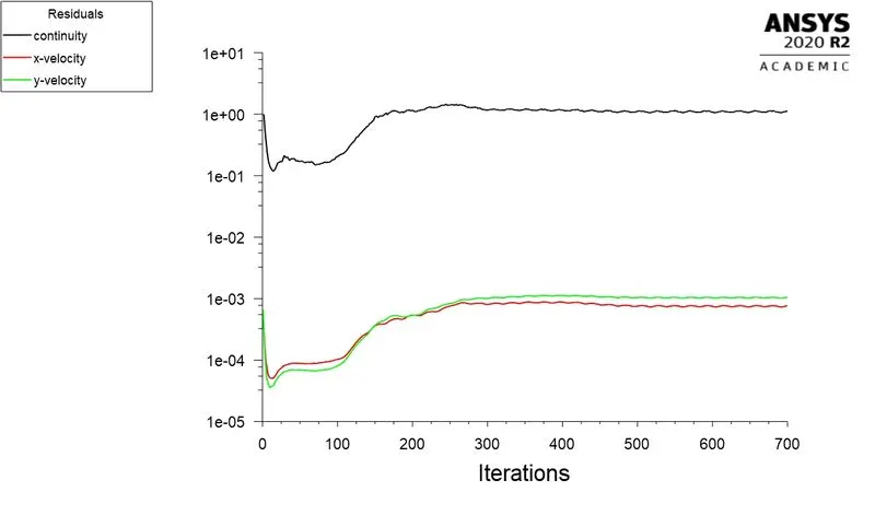
Residuals plot.
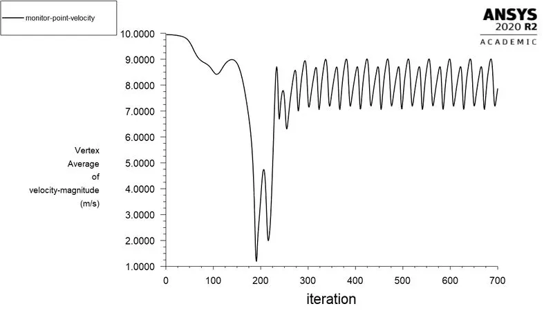
Monitor point velocity.
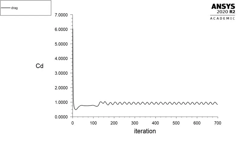
Drag coefficient plot.
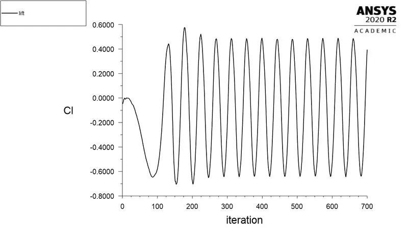
Lift coefficient plot.
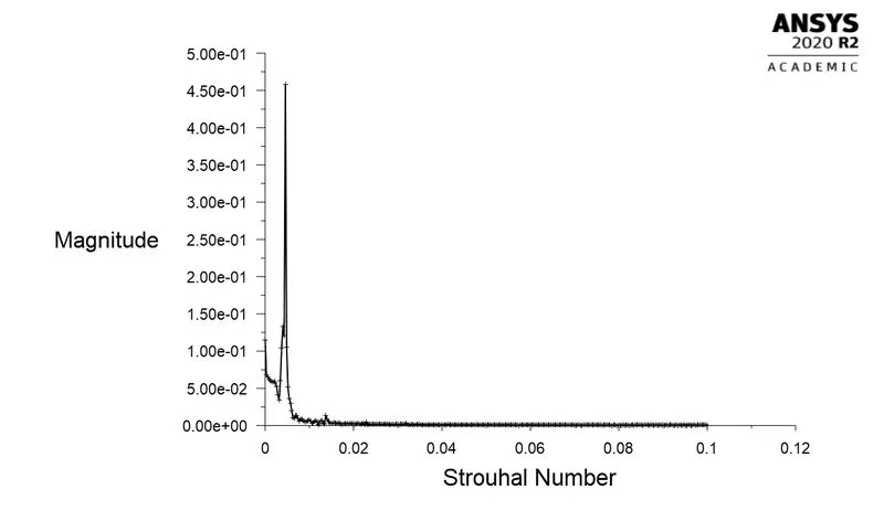
Spectral analysis of lift coefficient.
CASE 5.
Reynolds Number: 10000
Steady flow simulation.
Viscosity: 0.02
Density of the fluid:1 kg/m^3
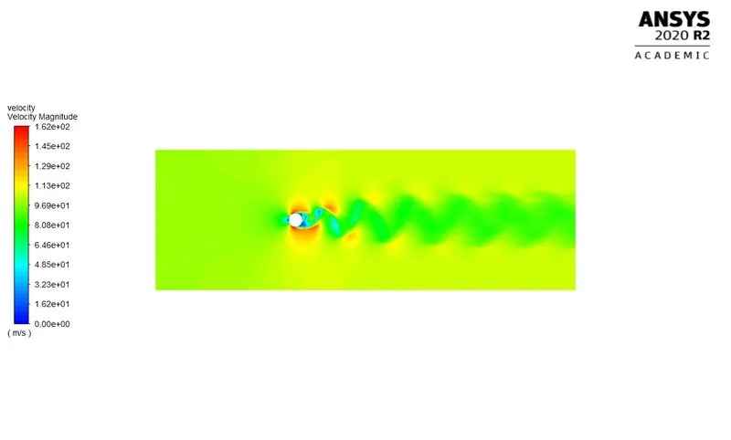
Velocity contour.
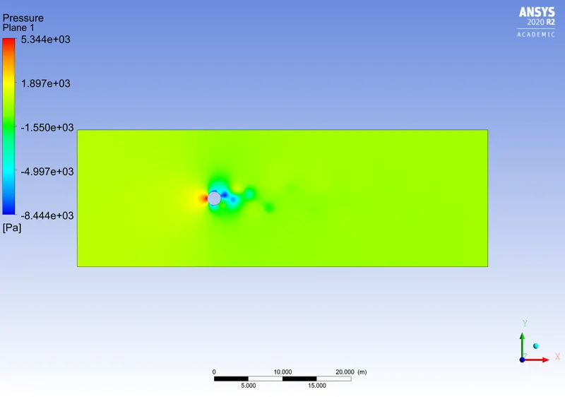
Pressure contour.
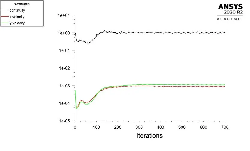
Residuals plot.
Monitor point velocity plot.
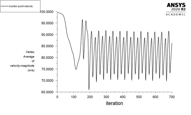
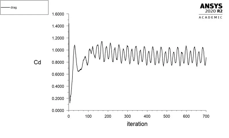
Drag coefficient plot.
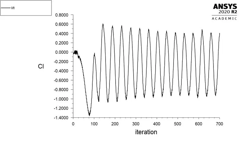
Lift coefficient plot.
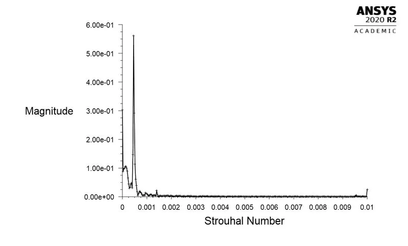
Spectral analysis of lift coefficient.
CASE 6.
Reynolds Number: 100000
Steady flow simulation.
Viscosity: 0.02
Density of the fluid:1 kg/m^3
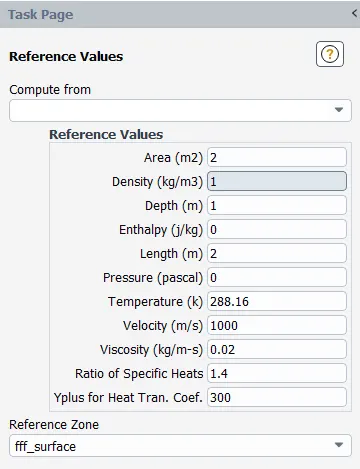
Velocity contour.
Pressure contour.
Residuals plot.
Monitor point velocity.
Drag coefficient.
Lift coefficient.
Spectral analysis of lift coefficient.
CONCLUSION.
| Reynolds Number | Cd | Cl |
|
10 |
3.367 | -0.00200315 |
|
100 |
1.3603 | -0.14512 |
|
1000 |
0.85989 | 0.39425 |
|
10000 |
0.8779 | 0.40707 |
|
100000 |
1.018126 | 0.02638 |
In the above table we can observe that as the Reynolds Number increases the drag coefficient is decreasing.