Week 2 Air standard Cycle

Otto Cycle:

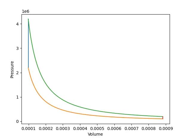
The processes which take place in otto cycle are

1. process 1-2 - reversible adiabatic (Isentropic) compression.

2. process 2-3 - constant volume heat addition.

3. process 3-4 - reversible adiabatic (Isentropic) Expansion.

4. process 4-1 - constant volume heat rejection.

The Python code starts with defining the engine kinematics function

The formula governing the engine kinematics is given by:

`V/V_c = 1 + 0.5(cr - 1)[R+1- costheta -(R^2 - sin^2theta)^0.5]`

The above formula corelates the Volume of the cylinder with respect to the crank angle. After defining the kinematics funtion, comes the input valiables, which includes the geometric parameters as well.

The vloume computation which includes the calculation of the pressure and the volume to yield the P-V diagram of the Otto Cycle.

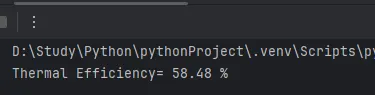
The complete python code is illustrated below, which yields the P-V plot as well as the thermal efficiency of the engine, which can be calculated by :

otto = `[1-1/(cr^(gamma-1))]*100`

import math
import matplotlib.pyplot as plt


def engine_kinematics(bore, stroke, con_rod, cr, start_crank, end_crank):

    # Geometric parameters

    a = stroke / 2
    R = con_rod / a

    # Volume parameters
    V_s = math.pi * (1 / 4) * pow(bore, 2) * stroke
    V_c = V_s / (cr - 1)

    sc = math.radians(start_crank)
    ec = math.radians(end_crank)

    num_values = 100

    dtheta = (ec - sc) / (num_values - 1)

    V = []

    for i in range(0, num_values):
        theta = sc + i * dtheta
        term1 = 0.5 * (cr - 1)
        term2 = R + 1 - math.cos(theta)
        term3 = pow(R, 2) - pow(math.sin(theta), 2)
        term3 = pow(term3, 0.5)

        V.append((1 + term1 * (term2 - term3)) * V_c)

    return V


# inputs
p1 = 101325
t1 = 500
gamma = 1.4
t3 = 2300

# geometric parameters
bore = 0.1
stroke = 0.1
con_rod = 0.15
cr = 9

# volume computation
V_s = (math.pi / 4) * pow(bore, 2) * stroke
V_c = V_s / (cr - 1)
v1 = V_c + V_s

# State point 2
v2 = V_c

# p2v2^gamma = p1v1^gamma
p2 = p1 * pow(v1, gamma) / pow(v2, gamma)

# p2v2/t2 = p1v1/t1 | t2 = p2*v2*t1/(p1*v1)
t2 = p2 * v2 * t1 / (p1 * v1)

V_compression = engine_kinematics(bore, stroke, con_rod, cr, 180, 0)
# P_compression*V_compression^gamma = constant
constant = p1 * pow(v1, gamma)

P_compression = []
for v in V_compression:
    P_compression.append(constant / pow(v, gamma))

# State point 3
v3 = v2

# p3v3/t3 = p2v2/t2 | p3 = p2*v2*t3/(t2*v3)
p3 = p2 * v2 * t3 / (t2 * v3)

V_expansion = engine_kinematics(bore, stroke, con_rod, cr, 0, 180)
# P_expansion*V_expansion^gamma = constant
constant = p3 * pow(v3, gamma)

P_expansion = []
for v in V_expansion:
    P_expansion.append(constant / pow(v, gamma))

# state point 4
v4 = v1

# p4v4^gamma = p3v3^gamma
p4 = p3 * pow(v3, gamma) / pow(v4, gamma)

# p4v4/t4 = p3*v3/t3 | t4 = p4*v4*t3/(p3*v3)
t4 = p4 * v4 * t3 / (p3 * v3)

# Thermal Efficiency for Otto cycle
eff = 1 - (1 / pow(cr, (gamma - 1)))
T_eff = eff * 100
print('Thermal Efficiency= %.2f %%' % (T_eff))

# Plotting for P-V Diagram
plt.plot([v2, v3], [p2, p3])
plt.plot(V_compression, P_compression)
plt.plot(V_expansion, P_expansion)
plt.plot([v4, v1], [p4, p1])
plt.xlabel('Volume')
plt.ylabel('Pressure')

plt.show()

Bearing the following graph of the Pressure V Volume.

The Thermal efficiency of the engine is calculated to be:

58.48%