Week 7 - Simulation of a 1D Supersonic nozzle flow simulation using Macormack Method
The main MATLAB code is below:
close all
clear all
clc

%Inputs
n = 31;         %No. of grid points
gamma = 1.4;
x = linspace(0,3,n);
dx = x(2) - x(1);
nt = 1400;      %No. of time step
C = 0.5;        %Courant Number

%% NON CONSERVATIVE FORM

[Mass_flow_rate_NC, Pressure_NC, Mach_number_NC, rho_NC, v_NC, T_NC, rho_throat_NC, v_throat_NC, T_throat_NC, Mass_flow_rate_throat_NC, Pressure_throat_NC, Mach_number_throat_NC] = NCF(x, dx, n, gamma, nt, C);

hold on

%Plots
figure(2)
%Timestep variation of properties at throat area (Non-Conservative form)

%Density
subplot(4,1,1)
plot(linspace(1,nt,nt),rho_throat_NC,'color','r', 'linewidth', 2)
ylabel('Density')
legend({'Density at throat'});
axis([0 1400 0 1.3]);
grid on;
title('NON CONSERVATIVE FORM')

%Temperature
subplot(4,1,2)
plot(linspace(1,nt,nt),T_throat_NC,'color','g', 'linewidth', 2)
ylabel('Temperature')
legend({'Temperature at throat'});
axis([0 1400 0.6 1]);
grid on;

%Pressure
subplot(4,1,3)
plot(linspace(1,nt,nt),Pressure_throat_NC,'color','b', 'linewidth', 2)
ylabel('Pressure')
legend({'Pressure at throat'});
axis([0 1400 0.4 1.1]);
grid on

%Mach Number
subplot(4,1,4)
plot(linspace(1,nt,nt),Mach_number_throat_NC,'color','k', 'linewidth', 2)
xlabel('Timesteps')
ylabel('Mach Number')
legend({'Mach Number at throat'});
axis([0 1400 0.6 1.4]);
grid on;


figure(3);
%Steady state simulation for primitve values (Non-Conservative form)

%Density
subplot(4,1,1);
plot(x,rho_NC,'color','r', 'linewidth', 2)
ylabel('Density')
legend({'Density'});
axis([0 3 0 1])
grid on;
title('NON CONSERVATIVE')

%Temperature
subplot(4,1,2);
plot(x,T_NC,'color','g', 'linewidth', 2)
ylabel('Temperature')
legend({'Temperature'});
axis([0 3 0 1])
grid on;

%Pressure
subplot(4,1,3);
plot(x,Pressure_NC,'color','b', 'linewidth', 2)
ylabel('Pressure')
legend({'Pressure'});
axis([0 3 0 1])
grid on;

%Mach number
subplot(4,1,4);
plot(x,Mach_number_NC,'color','k', 'linewidth', 2)
xlabel('Nozzle Length')
ylabel('Mach number')
legend({'Mach number'});
axis([0 3 0 4])
grid on;


%% CONSERVATIVE FORM

[Mass_flow_rate_C, Pressure_C, Mach_number_C, rho_C, v_C, T_C, rho_throat_C, v_throat_C, T_throat_C, Mass_flow_rate_throat_C, Pressure_throat_C, Mach_number_throat_C] = CF(x, dx, n, gamma, nt, C);


%Plots

figure(5)
%Timestep variation of properties at throat area (Conservative form)

%Density
subplot(4,1,1)
plot(rho_throat_C,'color','r', 'linewidth', 2)
ylabel('Density')
legend({'Density at throat'});
axis([0 1400 0 1]);
grid on;
title('CONSERVATIVE FORM')

%Temperature
subplot(4,1,2)
plot(T_throat_C,'color','g', 'linewidth', 2)
ylabel('Temperature')
legend({'Temperature at throat'});
axis([0 1400 0.6 1]);
grid on;

%Pressure
subplot(4,1,3)
plot(Pressure_throat_C,'color','b', 'linewidth', 2)
ylabel('Pressure')
legend({'Pressure at throat'});
axis([0 1400 0.2 0.8]);
grid on

%Mach Number
subplot(4,1,4)
plot(Mach_number_throat_C,'color','k', 'linewidth', 2)
xlabel('Timesteps')
ylabel('Mach Number')
legend({'Mach Number at throat'});
axis([0 1400 0.6 1.4]);
grid on;


figure(6);
%Steady state simulation for primitve values (Conservative form)

%Density
subplot(4,1,1);
plot(x,rho_C,'color','r', 'linewidth', 2)
ylabel('Density')
legend({'Density'});
axis([0 3 0 1])
grid on;
title('CONSERVATIVE FORM')

%Temperature
subplot(4,1,2);
plot(x,T_C,'color','g', 'linewidth', 2)
ylabel('Temperature')
legend({'Temperature'});
axis([0 3 0 1])
grid on;

%Pressure
subplot(4,1,3);
plot(x,Pressure_C,'color','b', 'linewidth', 2)
ylabel('Pressure')
legend({'Pressure'});
axis([0 3 0 1])
grid on;

%Mach number
subplot(4,1,4);
plot(x,Mach_number_C,'color','k', 'linewidth', 2)
xlabel('Nozzle Length')
ylabel('Mach number')
legend({'Mach number'});
axis([0 3 0 4])
grid on;


figure(7)
%Mass Flow Rate Comparison Plot

hold on
plot(x,Mass_flow_rate_NC,'r','linewidth',2)
hold on;
plot(x,Mass_flow_rate_C,'k','linewidth',2)
hold on;
grid on
legend('Non Conservative','Conservative');
xlabel('Length of the Domain')
ylabel('Mass Flow Rate')
title('Comparison of Mass Flow Rate of both forms')
The function MATLAB code for non conservative form is:
%% Non-Conservative form

function [Mass_flow_rate_NC, Pressure_NC, Mach_number_NC, rho_NC, v_NC, T_NC, rho_throat_NC, v_throat_NC, T_throat_NC, Mass_flow_rate_throat_NC, Pressure_throat_NC, Mach_number_throat_NC] = NCF(x, dx, n, gamma, nt, C)

%Intial boundary conditions

rho_NC = 1 - 0.3146*x;
T_NC = 1 - 0.2341*x;
v_NC = (0.1 + 1.09*x).*T_NC.^0.5;
a = 1 + 2.2*(x - 1.5).^2; %Area profile
throat = find(a==1); %Throat profile

%Outer Time Loop
for k = 1:nt

    %Time-step control
    dt = min(C.*dx./(sqrt(T_NC) + v_NC));

    %Saving a copy of Old Values
    rho_old = rho_NC;
    T_old = T_NC;
    v_old = v_NC;

   %Step 1 - Predictor method (forward difference for space terms)
    for j = 2:n-1

        %Simplifying the Equation's spatial terms
        dv_dx = (v_NC(j + 1) - v_NC(j))/dx;
        drho_dx = (rho_NC(j + 1) - rho_NC(j))/dx;
        dT_dx = (T_NC(j + 1) - T_NC(j))/dx;
        dlog_a_dx = (log(a(j + 1)) - log(a(j)))/dx;

        %Continuity Equation
        drho_dt_P(j) = -rho_NC(j)*dv_dx - rho_NC(j)*v_NC(j)*dlog_a_dx - v_NC(j)*drho_dx;

        %Momentum Equation
        dv_dt_P(j) = -v_NC(j)*dv_dx - (1/gamma)*(dT_dx + (T_NC(j)*drho_dx/rho_NC(j)));

        %Energy Equation
        dT_dt_P(j) = -v_NC(j)*dT_dx - (gamma - 1)*T_NC(j)*(dv_dx + v_NC(j)*dlog_a_dx);

        %Step 2 - Solution update
        rho_NC(j) = rho_NC(j) + drho_dt_P(j)*dt;
        v_NC(j) = v_NC(j) + dv_dt_P(j)*dt;
        T_NC(j) = T_NC(j) + dT_dt_P(j)*dt;

    end

    %Step 3 - Corrector method (backward difference for space terms)
    for j = 2:n-1

        %Simplifying the Equation's spatial terms
        dv_dx = (v_NC(j) - v_NC(j - 1))/dx;
        drho_dx = (rho_NC(j) - rho_NC(j - 1))/dx;
        dT_dx = (T_NC(j) - T_NC(j - 1))/dx;
        dlog_a_dx = (log(a(j)) - log(a(j - 1)))/dx;

        %Continuity Equation
        drho_dt_C(j) = - rho_NC(j)*dv_dx - rho_NC(j)*v_NC(j)*dlog_a_dx - v_NC(j)*drho_dx;

        %Momentum Equation
        dv_dt_C(j) = - v_NC(j)*dv_dx - (1/gamma)*(dT_dx + (T_NC(j)*drho_dx/rho_NC(j)));

        %Energy Equation
        dT_dt_C(j) = - v_NC(j)*dT_dx - (gamma - 1)*T_NC(j)*(dv_dx + v_NC(j)*dlog_a_dx);

    end

    %Step 4 - finding Average derivatives
    drho_dt = 0.5.*(drho_dt_P + drho_dt_C);
    dv_dt = 0.5.*(dv_dt_P + dv_dt_C);
    dT_dt = 0.5.*(dT_dt_P + dT_dt_C);

    %Step 5 - Final solution update
    for i = 2:n-1
        rho_NC(i) = rho_old(i) + drho_dt(i)*dt;
        v_NC(i) = v_old(i) + dv_dt(i)*dt;
        T_NC(i) = T_old(i) + dT_dt(i)*dt;
    end
    %Applying Boundary Conditions
    %At Inlet
    rho_NC(1) = 1;
    v_NC(1) = 2*v_NC(2) - v_NC(3);
    T_NC(1) = 1;

    %At Outlet
    rho_NC(n) = 2*rho_NC(n-1) - rho_NC(n - 2);
    v_NC(n) = 2*v_NC(n - 1) - v_NC(n - 2);
    T_NC(n) = 2*T_NC(n - 1) - T_NC(n - 2);

    %Defining Mass flow rate, Pressure and Mach number
    Mass_flow_rate_NC = rho_NC.*a.*v_NC;
    Pressure_NC = rho_NC.*T_NC;
    Mach_number_NC = (v_NC./sqrt(T_NC));

    %Calculating Variables at throat section
    rho_throat_NC(k) = rho_NC(throat);
    T_throat_NC(k) = T_NC(throat);
    v_throat_NC(k) = v_NC(throat);
    Mass_flow_rate_throat_NC(k) = Mass_flow_rate_NC(throat);
    Pressure_throat_NC(k) = Pressure_NC(throat);
    Mach_number_throat_NC(k) = Mach_number_NC(throat);

    %PLOTTING
    %Comparison of non-dimensional Mass flow rates at different time steps
    figure(1);
    if k == 50
       plot(x, Mass_flow_rate_NC, 'r', 'linewidth', 2);
       hold on
    elseif k == 100
       plot(x, Mass_flow_rate_NC, 'g', 'linewidth', 2);
       hold on
    elseif k == 200
       plot(x, Mass_flow_rate_NC, 'b', 'linewidth', 2);
       hold on
    elseif k == 400
       plot(x, Mass_flow_rate_NC, 'k', 'linewidth', 2);
       hold on
    elseif k == 800
       plot(x, Mass_flow_rate_NC, 'm', 'linewidth', 2);
       hold on
    elseif k == 1000
       plot(x, Mass_flow_rate_NC, 'c', 'linewidth', 2);
       hold on
    elseif k == 1400
       plot(x, Mass_flow_rate_NC, 'linewidth', 2);
       hold on
    end

    %Labelling
    title('NON CONSERVATIVE FORM')
    xlabel('Distance')
    ylabel('Mass flow rate')
    legend({'50^t^h Timestep','100^t^h Timestep','200^t^h Timestep','400^t^h Timestep','800^t^h Timestep','1000^t^h Timestep','1400^t^h Timestep'})
    axis([0 3 0 2])
    grid on

end

end
The function MATLAB code for conservative form is:
%% Conservative form

function [Mass_flow_rate_C, Pressure_C, Mach_number_C,  rho_C, v_C, T_C, rho_throat_C, v_throat_C, T_throat_C, Mass_flow_rate_throat_C, Pressure_throat_C, Mach_number_throat_C] = CF(x, dx, n, gamma, nt, C)

%Determining Initial profile of Density and Temperature
for i = 1:n

    if (x(i) >= 0 && x(i) <= 0.5)
        rho_C(i) = 1;
        T_C(i) = 1;
    elseif (x(i) >= 0.5 && x(i) <= 1.5)
        rho_C(i) = 1 - 0.366*(x(i) - 0.5);
        T_C(i) = 1 - 0.167*(x(i) - 0.5);
    elseif (x(i) >= 1.5 && x(i) <= 3)
        rho_C(i) = 0.634 - 0.3879*(x(i) - 1.5);
        T_C(i) = 0.833 - 0.3507*(x(i) - 1.5);
    end

end

a = 1 + 2.2*(x - 1.5).^2; %Area profile
throat = find(a==1); %Throat profile

%Initial profile fot Velocity and Pressure
v_C = 0.59./(rho_C.*a);
Pressure_C = rho_C.*T_C;

%Calculate the Initial Solution Vectors(U)
U1 = rho_C.*a;
U2 = rho_C.*a.*v_C;
U3 = rho_C.*a.*(T_C./(gamma - 1)) + ((gamma/2).*v_C.^2);

%Outer Time Loop
for k =1:nt

    %Time-step control
    dt = min(C.*dx./(sqrt(T_C) + v_C));

    %Saving a copy of Old Values
    U1_old = U1;
    U2_old = U2;
    U3_old = U3;

    %Calculating the Flux vector(F)
    F1 = U2;
    F2 = ((U2.^2)./U1) + ((gamma - 1)/gamma)*(U3 - (gamma/2)*((U2.^2)./U1));
    F3 = ((gamma*U2.*U3)./U1) - (gamma*(gamma - 1)*((U2.^3)./(2*U1.^2)));

    %Step 1 - Predictor method (forward difference for space terms)
    for j = 2:n-1

        %Calculating the Source term(J)
        J2(j) = (1/gamma)*rho_C(j)*T_C(j)*((a(j + 1) - a(j))/dx);


        %Continuity Equation
        dU1_dt_P(j) = -((F1(j + 1) - F1(j))/dx);

        %Momentum Equation
        dU2_dt_P(j) = -((F2(j + 1) - F2(j))/dx) + J2(j);

        %Energy Equation
        dU3_dt_P(j) = -((F3(j + 1) - F3(j))/dx);

        %Step 2 - Solution update
        U1(j) = U1(j) + dU1_dt_P(j)*dt;
        U2(j) = U2(j) + dU2_dt_P(j)*dt;
        U3(j) = U3(j) + dU3_dt_P(j)*dt;

    end

    %Updating Flux vectors
    F1 = U2;
    F2 = ((U2.^2)./U1) + ((gamma - 1)/gamma)*(U3 - ((gamma*0.5*(U2.^2))./(U1)));
    F3 = ((gamma*U2.*U3)./U1) - ((gamma*0.5*(gamma - 1)*(U2.^3))./(U1.^2));

   %Step 3 - Corrector method (backward difference for space terms)
    for j = 2:n-1

        %Updating the Source term(J)
        J2(j) = (1/gamma)*rho_C(j)*T_C(j)*((a(j) - a(j - 1))/dx);

        %Simplifying the Equation's spatial terms
        dU1_dt_C(j) = -((F1(j) - F1(j - 1))/dx);
        dU2_dt_C(j) = -((F2(j) - F2(j - 1))/dx) + J2(j);
        dU3_dt_C(j) = -((F3(j) - F3(j - 1))/dx);

    end

    %Step 4 - finding Average derivatives
    dU1_dt = 0.5*(dU1_dt_P + dU1_dt_C);
    dU2_dt = 0.5*(dU2_dt_P + dU2_dt_C);
    dU3_dt = 0.5*(dU3_dt_P + dU3_dt_C);

    %Step 5 - Final solution update
    for i = 2:n-1
        U1(i) = U1_old(i) + dU1_dt(i)*dt;
        U2(i) = U2_old(i) + dU2_dt(i)*dt;
        U3(i) = U3_old(i) + dU3_dt(i)*dt;

    end

    %Applying Boundary Conditions
    %At Inlet
    U1(1) = rho_C(1)*a(1);
    U2(1) = 2*U2(2) - U2(3);

    v_C(1) = U2(1)./U1(1);
    U3(1) = U1(1)*((T_C(1)/(gamma - 1)) + ((gamma/2)*(v_C(1)).^2));

    %At Outlet
    U1(n) = 2*U1(n - 1) - U1(n - 2);
    U2(n) = 2*U2(n - 1) - U2(n - 2);
    U3(n) = 2*U3(n - 1) - U3(n - 2);

    %Final Primitive value update
    rho_C = U1./a;
    v_C = U2./U1;
    T_C = (gamma - 1)*((U3./U1 - (gamma/2)*(v_C).^2));

    %Defining Mass flow rate, Pressure and Mach number
    Mass_flow_rate_C = rho_C.*a.*v_C;
    Pressure_C = rho_C.*T_C;
    Mach_number_C = (v_C./sqrt(T_C));

    %Calculating Variables at throat section
    rho_throat_C(k) = rho_C(throat);
    T_throat_C(k) = T_C(throat);
    v_throat_C(k) = v_C(throat);
    Mass_flow_rate_throat_C(k) = Mass_flow_rate_C(throat);
    Pressure_throat_C(k) = Pressure_C(throat);
    Mach_number_throat_C(k) = Mach_number_C(throat);

    %PLOTTING
    %Comparison of non-dimensional Mass flow rates at different time steps
    figure(4)
    if k == 50
       plot(x, Mass_flow_rate_C, 'r', 'linewidth', 2);
       hold on
    elseif k == 100
       plot(x, Mass_flow_rate_C, 'g', 'linewidth', 2);
       hold on
    elseif k == 200
       plot(x, Mass_flow_rate_C, 'b', 'linewidth', 2);
       hold on
    elseif k == 400
       plot(x, Mass_flow_rate_C, 'k', 'linewidth', 2);
       hold on
    elseif k == 800
       plot(x, Mass_flow_rate_C, 'm', 'linewidth', 2);
       hold on
    elseif k == 1000
       plot(x, Mass_flow_rate_C, 'c', 'linewidth', 2);
       hold on
    elseif k == 1400
       plot(x, Mass_flow_rate_C, 'linewidth', 2);
       hold on
    end

    %Labelling
    title('CONSERVATIVE FORM')
    xlabel('Distance')
    ylabel('Mass flow rate')
    legend({'50^t^h Timestep','100^t^h Timestep','200^t^h Timestep','400^t^h Timestep','800^t^h Timestep','1000^t^h Timestep','1400^t^h Timestep'})
    axis([0 3 0.4 1])
    grid on

end

end
The function code consists of 5 steps:
- initial conditions
- predictor step
- solution update
- correction step
- averaging step
- final solution update
Boundary conditions are applied to the loop to yield the Mass Flow Rate, Mach Number, and the Pressure. The solution outputs are dipicted below. Grid independent test implies the optimum mesh size for the solution. The solutions since almost remain same for the 'n values' the solutions is a grid indepentant.
- Steady-state distribution of primitive variables inside the nozzle
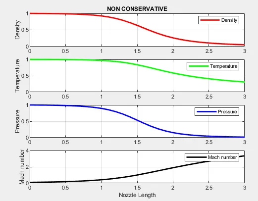
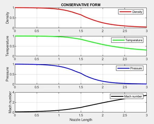
The graphs of the primitive variables inside the nozzle in both the forms highlights the same results for the total length of the nozzle.
- Time-wise variation of the primitive variables
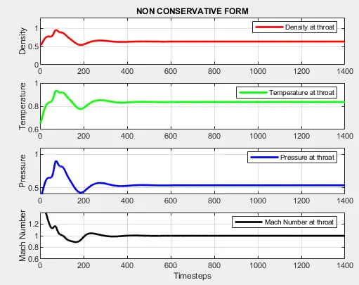
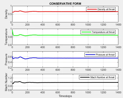
From the above graphs it is clear that for the non conservative form the values fluctuate for a bit attaining stability compared to conservative form.
- Variation of Mass flow rate distribution inside the nozzle at different time steps during the time-marching process
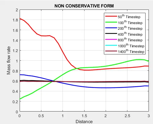
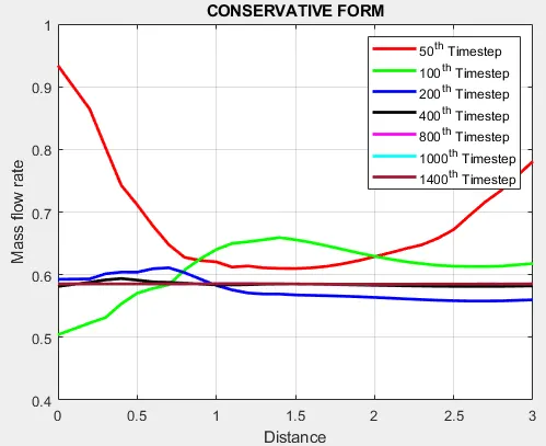
The above illustrated graphs for the 2 forms shows that at about `400^(th)` step the solutions attain stability till the entire domain. The graph of conservative form shows a bit more stability as compared to the non-conservative form.
- Comparison of Normalized mass flow rate distributions of both forms
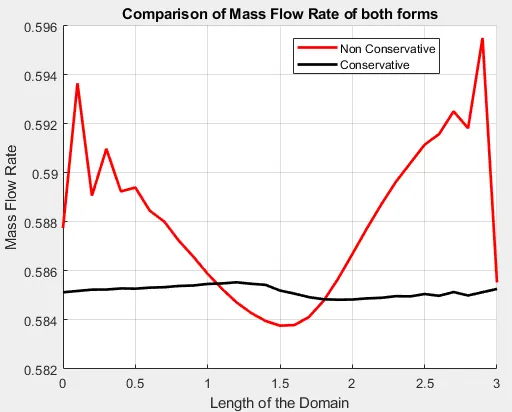
The graphs below illustrates that although the final solutions are similar, but the conservative form is more stable compared to non-conservative form, and yields the comparitively stable results throughout the length of the nozzle.