Assignment 2

Assignment 2:

Questions:

1. 1. Check the material properties of the rail component and calculate the speed of sound in steel rail=_______
2. 2. The length of the rail is about 1000 mm. Calculate the time takes for a shock wave to travel from one end of the rail to the other.
3. 3. Time for sound to travel length of rail=______
4. 4. Edit the engine file so that the stress wave can be monitored, moving from one end of the rail to the other during impact -this will require a termination time equal to the time it takes for the sound to travel the length of the rail(set on/RUN card)
5. 5. Set the frequency of animation output to a time that will give 20 animation steps (/ANIM/DT)
6. 6. Change /print -10.
7. 7. 3D meshing tetra mesh and hex mesh

• Repeat class examples and, maintain the quality.
• Target tet size=5mm, hex size=10mm, tet collapse=0.15.

Solutions 1. The material properties of the rail component can be obtained through the file named ‘FIRST_RUN_0000.rad’, and is shown in the figure below.

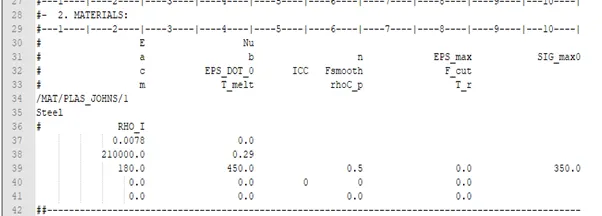
Figure ‑1 Material Properties for the JOHNSON-COOK Material

To calculate the speed of sound in steel rail the following formula is used as described in the equation below.

`∆t_e=l/c=l/√(E⁄ρ)` ......... Equation -1

Where,

_{`∆t_e`}is elemental time step

l is the length of the element

E is Young’s modulus of the material

`ρ` is the density of the material

Hence, `c=√(E/ρ)` ........ Equation -2

Putting the values of E and `ρ` of 210,000 MPa and 0.0078 x10³ Kg/l in Equation -2, we get the value of c to be 5188 m/sec.

Solutions 2. Since the speed of sound is 5188m/sec, using Equation -1 the `∆t_e` is calculated to be about 0.19ms.

Solutions 3. The time taken for the sound to travel a length of 1m is about 0.2msec.

Solutions 4. The engine file can be edited through importing the ‘FIRST_RUN_0000.rad’ and editing the run time to the value calculated in Solution 2 using Equation -1.

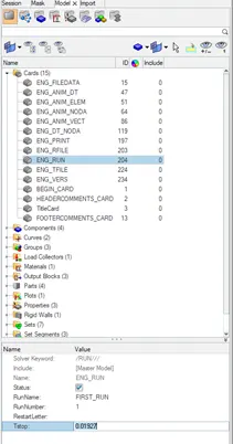
Figure ‑2 Modified Tstop

Solutions 5. As the mentioned animation step is indicated to be 20. Hence, the frequency of animation or T_freq is 0.01927/20 = 0.0009365 msec. Now the value for the same can be changed in ‘ENG_ANIM_DT’, as shown below.

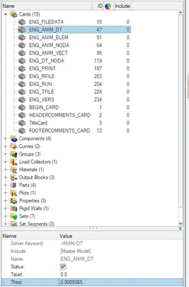
Figure ‑3 Modified Tfreq

Solutions 6. Exporting the card of ‘ENG_PRINT’, we can open it and change the /PRINT values, as shown in the figure.

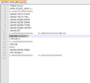
Figure -4 Snippet of the Engine file

Solutions 7.

Arm_Bracket

The geometry model under consideration is illustrated in the figure below.

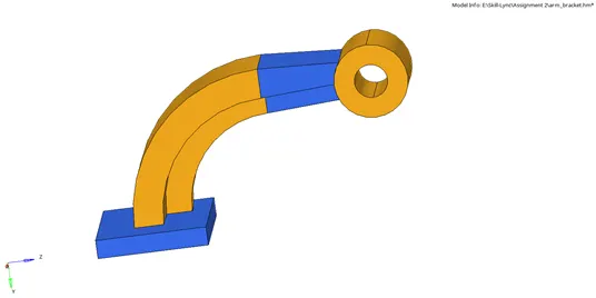
Figure ‑5 The model

The meshing starts from the base, with the element offsetting the 2D generated mesh with the element size of 10mm to the distance of 25mm. The figure below illustrates the meshing of the base.

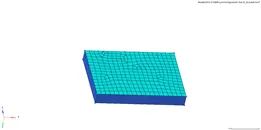
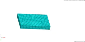
Figure ‑6 2D generated mesh on the top surface of the base Figure ‑7 The final mesh of the base

Now for the arm curve, which is quarter circular, the meshing starts with ‘Hexa’ elements and ‘spin element’ feature. The common elements between the base and the arm curve are selected which is performed by masking the rest of the 3D elements of the arm bracket, now the centre of the arc is selected for the normal vector for a total 90° spin, as shown in the figures below.

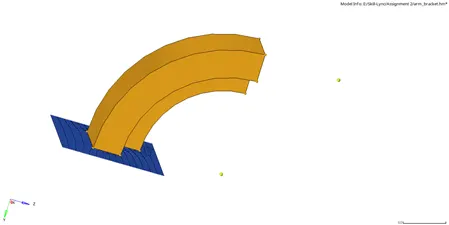
Figure ‑8 The masked 3D HEXA elements

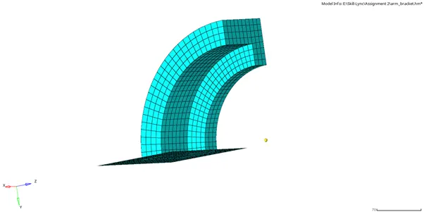
Figure ‑9 The generated mesh for the arm curve

The next part is the arm straight, which is an extension of the arm curve. The meshing starts with 'linear solid' feature. The figure below shows the part to be meshed.

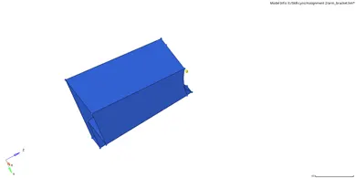
Figure ‑10 The arm straight geometry

For the linear solid feature, the face mesh was generated on the common face to the arm curve and arm straight. The face mesh was extended maintaining the number of elements and alignment intact, as shown in the figure below.

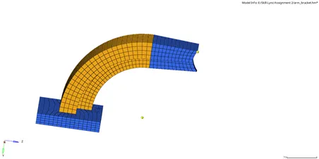
Figure ‑11 The final mesh of the arm straight

For the boss part of the geometry, one surface was meshed following the element concentration on the arm straight. Then the mesh was propagated using the ‘solid map’ feature, as illustrated in the figure below.

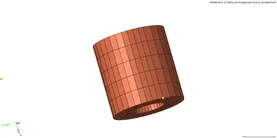
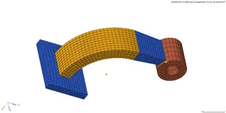
Figure ‑12 The final mesh of the boss Figure ‑13 The final mesh of the arm bracket

Housing

The housing consists of the cover and the hub geometry.

Starting with the hub, The hub was initially ‘tri’ elements were generated using the 2D mesh with the size of 5mm. Then the elements were propagated using ‘tetramesh’ feature for the 3D meshing. The tet collapse was checked for 0.15, and the figure below depicts the meshed hub.

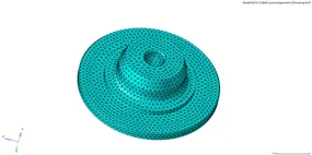
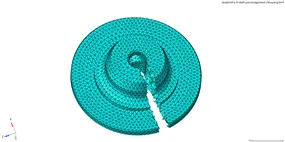
Figure ‑14 The Final mesh of the Hub component Figure ‑15 The 3D mesh with masked few elements

Now for the covering, a similar method is being carried out to obtain the results illustrated in the following figures.

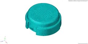
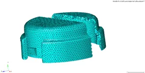
Figure ‑14 The Final mesh of the cover component Figure ‑15 The 3D mesh with masked few elements