Week 5.1 - Mid term project - Solving the steady and unsteady 2D heat conduction problem

The 2D heat conduction equation is given by:

`(∂T)/(∂t)=α((∂^2 T)/(∂x^2 )+(∂^2 T)/(∂y^2 ))` -Eqn(1)

As per the situation mentioned;

Temperature at the top boundary (`T_T`) is 600k

Temperature at the bottom boundary (`T_B`) is 900k

Temperature at the left boundary (`T_L`) is 400k

Temperature at the right boundary (`T_R`) is 800k

CASE-1

Firstly for the steady state:

The above equation (1) now can be rewritten as:

`((∂^2 T)/(∂x^2 )+(∂^2 T)/(∂y^2 ))=0` -Eqn(2)

Now the temperature at a point 'P' can be written as:

`T_P = (1/k)(Term_1 + Term_2)`

Where;

`k = 2((∆x^2+∆y^2)/(∆x^2*∆y^2 ))`

and the `Term_1 = ((T_L+T_R))/(∆x^2 )` `Term_2 = ((T_T+T_B))/(∆y^2 )`

The `T_P` can be calculated following 3 solvers:

• Jacobi
• Gauss-seidel
• Successive over-relaxation

The MATLAB code for solving the equation2 using the 3 different solvers is shown below.

%% Steady State 2D heat conduction problem

clc

%% Inputs

nx = 10;
ny = 10;
t = 300*ones(nx, ny);
t(1:nx, 1)  = 400;
t(1, 1:ny)  = 600;
t(1:nx, ny) = 800;
t(nx, 1:ny) = 900;

%Assuming grid temperature values
t(2:nx-1,2:ny-1) = 300;

%Assigning Corner temperature values
t(1,1) = (t(1,2)+t(2,1))/2;             
t(nx,1) = (t(nx-1,1)+t(nx,2))/2;        
t(1,ny) = (t(1,ny-1)+t(2,ny))/2;        
t(nx,ny) = (t(nx-1,ny)+t(nx,ny-1))/2;   
                 

error = 9e9;                            
tolerance = 1e-4;                       
x = linspace(0,1,nx);
y = linspace(0,1,ny);
dx = 1/(nx-1);
dy = 1/(ny-1);
k = 2*(dx^2 + dy^2)/(dx^2 * dy^2);
told = t;
omega = 1.1;

%% Selecting method to solve Steady State Problem

solver = input('ITERATIVE SOLVERS:\n1. Jacobi \n2. Gauss-Seidel \n3. Successive Over-Relaxation \n \nSelect the method to solve the Steady State problem: ');

%% JACOBI METHOD

if solver==1
    % Convergence Loop
    jacobi_iteration = 1;
    while error>tolerance
        % Space Loop
        for i = 2:nx-1
            for j = 2:ny-1
                term1 = (told(i-1,j)+told(i+1,j))/(dx^2);
                term2 = (told(i,j-1)+told(i,j+1))/(dy^2);
                t(i,j) = (term1+term2)/k;
            end
        end
        error = max(max(abs(told-t)));
        told = t;
        jacobi_iteration = jacobi_iteration +1;
    end

    fprintf('Number of Iterations for Jacobi Method = %d', jacobi_iteration);

    % Plot for JACOBI METHOD
    figure(1)
    contourf(x,y,t,'showtext','on')
    colormap(jet)
    colorbar
    set(gca,'YDIR','reverse')
    xlabel('X Domain')
    ylabel('Y Domain')
    title(sprintf('Steady State Analysis using JACOBI METHOD'))

end

%% GAUSS-SEIDEL

if solver==2
    % Convergence Loop
    gs_iteration = 1;
    while error>tolerance
        % Space Loop
        for i = 2:nx-1
            for j = 2:ny-1
                term1 = (t(i-1,j)+told(i+1,j))/(dx^2);
                term2 = (t(i,j-1)+told(i,j+1))/(dy^2);
                t(i,j) = (term1+term2)/k;
            end
        end
        error = max(max(abs(told-t)));
        told = t;
        gs_iteration = gs_iteration +1;
    end
    fprintf('Number of Iterations for Gauss-Seidel Method = %d', gs_iteration)
    %Plot for Gauss-seidel
    contourf(x,y,t,'showtext','on')
    colormap(jet)
    colorbar
    set(gca,'YDIR','reverse')
    xlabel('X Domain')
    ylabel('Y Domain')
    title(sprintf('Steady State Analysis using GAUSS-SEIDEL METHOD'))

end

%% Code for Successive over-relaxation

if solver==3
    % Convergence Loop
    sor_iteration = 1;
    while error>tolerance
        %Space Loop
        for i = 2:nx-1
            for j = 2:ny-1
                term1 = (t(i-1,j)+told(i+1,j))/(dx^2);
                term2 = (t(i,j-1)+told(i,j+1))/(dy^2);
                t_gs(i,j) = (term1+term2)/k;
                t(i,j) = (1-omega)*told(i,j) + omega*t_gs(i,j);
            end
        end
        diff = abs(told-t);
        error = max(max(diff));
        told = t;
        sor_iteration = sor_iteration +1;
    end
    fprintf('Number of Iterations for Successive over-relaxation method = %d', sor_iteration)
    %Plot for Successive over-relaxation
    contourf(x,y,t,'showtext','on')
    colormap(jet)
    colorbar

    set(gca,'YDIR','reverse')
    xlabel('X Domain')
    ylabel('Y Domain')
    title(sprintf('Steady Analysis using Successive Over Relaxation Method'))
end

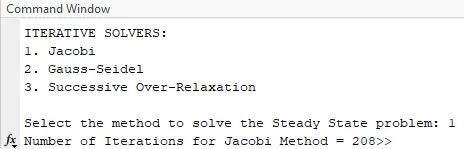
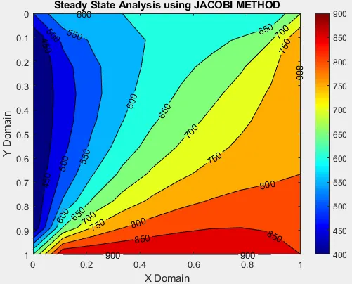
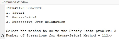
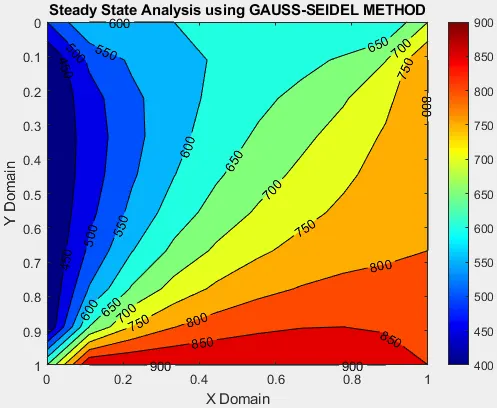
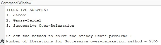
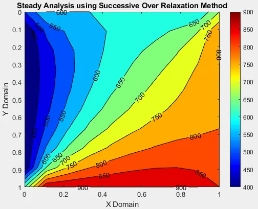
The number of iterations and the temperature contour graph corresponding to the respective solver is attached alongwith.

Jacobi Method

Gauss-Seidel Method

Successive over-relaxation Method

CASE-2

Secondly, for the transient state, the equation can be solved following the explicit method or implicit method.

• Explicit Method:

The temperature at a point P (`T_P`) as obtained by eqn (1) is:

`T_P = (T_P)_o + k_1*(Term_1)_o +k_2*(Term_2)_o`

Where;

`(T_P)_o` is the previous value of the `T_P`

`k_1 = (α/_\t)/(/_\x^2)`

`k_2 = (α/_\t)/(/_\y^2)`

`(Term_1)_o = (T_L -2(T_P) + T_R)_o`

`(Term_2)_o = (T_T -2(T_P) + T_B)_o`

• Implicit Method:

The temperature at a point P (`T_P`) as obtained by eqn (1) is:

`T_P = (1/(1+2k_1+2k_2))*[(T_P)_o + k_1(T_L+T_R) + k_2(T_T+T_B)]`

Where;

`(T_P)_o` is the previous value of the `T_P`

`k_1 = (α/_\t)/(/_\x^2)`

`k_2 = (α/_\t)/(/_\y^2)`

The MATLAB code solving both the explicit and the implicit method is:

%% Transient State 2D heat conduction problem

clc

%% Inputs

nx = 10;
ny = 10;
t = 300*ones(nx, ny);
t(1:nx, 1)  = 400;
t(1, 1:ny)  = 600;
t(1:nx, ny) = 800;
t(nx, 1:ny) = 900;

%Assuming grid values
t(2:nx-1,2:ny-1) = 300;  

%Assigning Corner temperature values 
t(1,1) = (t(1,2)+t(2,1))/2;             
t(nx,1) = (t(nx-1,1)+t(nx,2))/2;        
t(1,ny) = (t(1,ny-1)+t(2,ny))/2;        
t(nx,ny) = (t(nx-1,ny)+t(nx,ny-1))/2; 

told = t;
tprev = t;
error = 9e9;
tolerance = 1e-4;
x = linspace(0,1,nx);
y = linspace(0,1,ny);
dx = 1/(nx-1);
dy = 1/(ny-1);
dt = 1e-4;
alpha = 1.4;
omega = 1.01; 
k1 = (alpha*dt)/(dx^2);
k2 = (alpha*dt)/(dy^2);

%% Selecting method to solve Transient State Problem
solver = input('ITERATIVE SOLVERS:\n1. Explicit \n2. Implicit Jacobi \n3. Implicit Gauss-seidel \n4. Implicit Successive over-relaxation \n \nSelect the method to solve the Transient State problem: ');

%% For Explicit Method
if solver==1
        explicit_iteration = 1;
        while (error>tolerance)
            % Space Loop
            for i = 2:nx-1
                for j = 2:ny-1
                    term1=told(i,j);
                    term2 = k1*(told(i-1,j)-2*told(i,j)+told(i+1,j));
                    term3 = k2*(told(i,j+1)-2*told(i,j)+told(i,j-1));
                    t(i,j) = term1+term2+term3;
                end
            end
        error = max(max(abs(told-t)));
        told = t;
        explicit_iteration = explicit_iteration +1;
        end
    fprintf('Number of Iterations for Explicit Method = %d', explicit_iteration);
    figure(1)
    contourf(x,y,t,'showtext','on')
    colormap(jet)
    colorbar
    set(gca,'YDIR','reverse')
    xlabel('X Domain')
    ylabel('Y Domain')
    title(sprintf('Transient Analysis using EXPLICIT METHOD'))
    
end


%% Implicit Jacobi Method

if solver == 2
    iteration_implicit_jacobi = 1;
    term1 = 1/(1+2*k1+2*k2);
    term2 = k1*term1;
    term3 = k2*term1;
    for nt = 1:1400
        error = 9e9;
        while(error>tolerance)
            % Space Loop
            for i = 2:nx-1
                for j = 2:ny-1
                    H = told(i-1,j)+told(i+1,j);
                    V = told(i,j-1)+told(i,j+1);
                    t(i,j) = term1*tprev(i,j) + term2*H + term3*V;
                end
            end
            diff = abs(told-t);
            error = max(max(diff));
            told = t;
            iteration_implicit_jacobi = iteration_implicit_jacobi + 1;
        end
        tprev = t;
    end
    fprintf('Number of Iterations for Implicit Jacobi Method = %d', iteration_implicit_jacobi)
    contourf(x,y,t,'showtext','on')
    colormap(jet)
    colorbar
    set(gca,'YDIR','reverse')
    xlabel('X Domain')
    ylabel('Y Domain')
    title(sprintf('Transient Analysis using IMPLICIT JACOBI METHOD'))
end

%% Implicit Gauss-Seidel Method
if solver == 3
    iteration_implicit_GS = 1;
    term1 = 1/(1+2*k1+2*k2);
    term2 = k1*term1;
    term3 = k2*term1;
        for nt = 1:1400
            error  = 9e9;
            while(error>tolerance)
                % Space Loop
                for i = 2:nx-1
                    for j = 2:ny-1
                        H = t(i-1,j)+t(i+1,j);
                        V = t(i,j-1)+t(i,j+1);
                        t(i,j) = term1*tprev(i,j) + term2*H + term3*V;
                    end
                end
            iteration_implicit_GS = iteration_implicit_GS + 1;
            diff = abs(told-t);
            error = max(max(diff));
            told = t;
            end
        tprev = t;
        end

    fprintf('Number of Iterations for Implicit Gauss-Seidel Method = %d', iteration_implicit_GS)
    contourf(x,y,t,'showtext','on')
    colormap(jet)
    colorbar
    set(gca,'YDIR','reverse')
    xlabel('X Domain')
    ylabel('Y Domain')
    title(sprintf('Transient Analysis using IMPLICIT GAUSS-SEIDEL METHOD'))
end

%% For Implicit SOR Method
if solver == 4
    iteration_implicit_SOR = 1;
    term1 = 1/(1+2*k1+2*k2);
    term2 = k1*term1;
    term3 = k2*term1;
    for nt = 1:1400
        error = 9e9;
        while(error>tolerance)
            % Space Loop
            for i = 2:nx-1
                for j = 2:ny-1
                    H = t(i-1,j)+t(i+1,j);
                    V = t(i,j-1)+t(i,j+1);
                    t_gs(i,j) = term1*tprev(i,j) + term2*H + term3*V;
                    t(i,j) = (1-omega)*told(i,j) + omega*t_gs(i,j);
                end
            end
            iteration_implicit_SOR = iteration_implicit_SOR + 1;
            diff = abs(told-t);
            error = max(max(diff));
            told = t;
        end
        tprev = t;
    end
    fprintf('Number of Iterations for Implicit SOR = %d', iteration_implicit_SOR)
    contourf(x,y,t,'showtext','on')
    colormap(jet)
    colorbar
    set(gca,'YDIR','reverse')
    xlabel('X Domain')
    ylabel('Y Domain')
    title(sprintf('Transient Analysis using IMPLICIT SOR METHOD'))
end

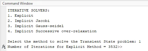
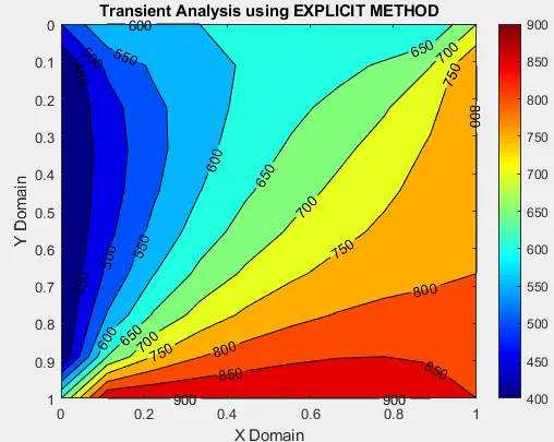
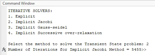
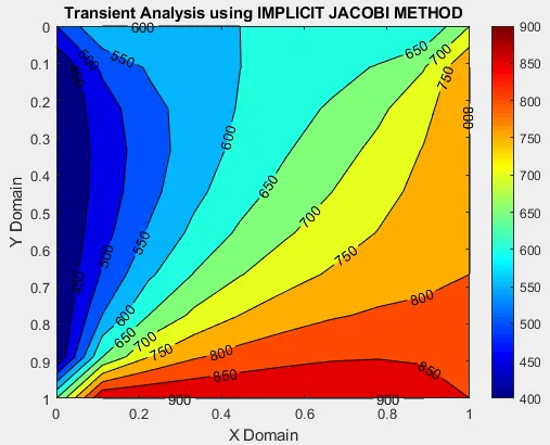
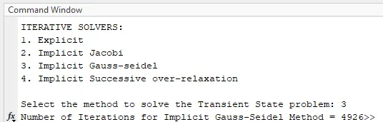
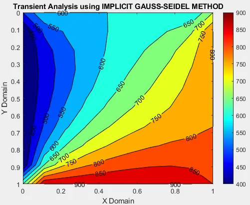
The number of iterations and the temperature contour graph corresponding to the respective solver is attached alongwith.

Explicit Method

Implicit Jacobi Method

Implicit Gauss-seidel Method

Implicit Successive over-relaxation Method

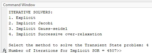
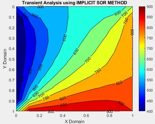
Now, from the above 7 countour graphs for 3 steady state analysis and 4 transient state analysis, it is evident that number of iterations is lower for the steady state analysis and among which the SOR bears the lowest number of iterations to converge the solution. The transient state analysis shows that explicit analysis converges the solution in a lesser number of iterations. Else for both steady state and transient state, jacobian converges at a greater time than Gauss-siedel and SOR converges at even lower number of iterations.