Assignment 4
Objective:
Compare seven cases as discussed in the last three slides, in a tabulated format on the basis of:
1. Total number of cycles, Energy error, mass error and simulation time.
2. Notice the animation of all five and describe the animations in brief, on the
basis of whether the elements are being deleted or cracked.
3. Plot energies and notice any difference.
4. Based on all the results, which case would represent the on-field
scenario.
5. Prepare a ppt/docx and list down case by case result and your conclusion
as to why the failure happened.
Solution:
Case 1: Law2_epsmax_failure
The model in ‘FAILURE_JOHNSON_0000.rad’ file was solved using the property card as depicted below, with a failure plastic strain of 0.151.
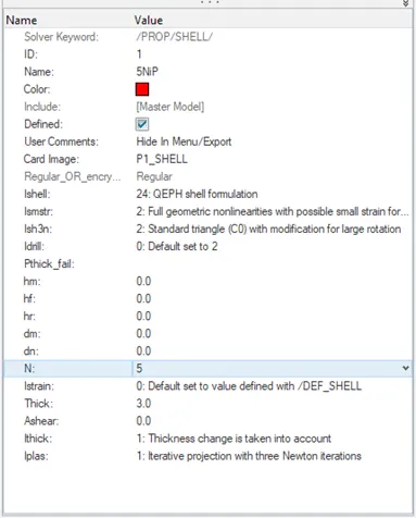
Figure -1 The property card of Case 1
Case 2: Law2_epsmax_crack
The model was then solved using the following parameters
| Parameters | Note |
| Lfail_sh=1 | Shell is deleted or cracked when `D=∑(∆ε_p)/ε_f ≥1` |
| Dadv=1 | Only active if Ixfem=1 |
| Ixfem=1 | Element crack formation |
Case 3: Law2_epsmax_nofail
Then, the model is run by deleting the /Fail/JOHNSON card.
Case 4: Law2
The next case is carried out by deleting the eps_p_max value from the above model.
Case 5: Law1
The model is then run by changing the material card to ‘M1_ELAST’ as shown in the figure below.
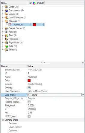
Figure -2 The snippet showing the material card
Case 6: Law27
Opening the file ‘LAW27_0000.rad’ the property card is modified to the recommended values, as illustrated in Figure -1 and then the material card is checked and the figure below depicts it.
Figure -3 The material card for Case 6
Case 7: Law36
The file ‘FAILURE_JOHNSON_0000.rad’ is again opened. The values of the parameters below were modified in the material.
|
Parameters |
Values |
|
Rho_initial |
0.0027 |
|
E |
71000 |
|
Nu |
0.33 |
|
Eps_p_max (failure plastic strain) |
0.16 |
|
EPS_t (tensile failure strain at which stress starts to reduce) |
0.1 |
|
EPS_m (maximum tensile failure strain at which the stress in the element is set to zero) |
0.11 |
Then the curve of stress-strain data, as tabulated below is assigned to the material using ‘fct_ID’.
|
Strain |
Stress (MPa) |
|
0 |
300 |
|
4.84405e-4 |
360.13 |
|
0.00111878 |
390.56 |
|
0.0032105 |
442.82 |
|
0.00478134 |
465.98 |
Comparison:
The table below shows the comparison of the cases with respect to no. of cycles, error in energy, error in mass, and finally
|
Case |
Total number of cycles |
Energy error |
Mass error |
Simulation Time |
|
Law2_epsmax_failure |
49380 |
0.80% |
0 |
105.52 |
|
Law2_epsmax_crack |
49217 |
4.10% |
0 |
114.74 |
|
Law2_epsmax_nofail |
49408 |
0.80% |
0 |
119.37 |
|
Law2 |
48737 |
3.00% |
0 |
115.06 |
|
Law1 |
47969 |
1.30% |
0 |
110.71 |
|
Law27 |
49508 |
0.80% |
0 |
131.98 |
|
Law36 |
53202 |
-1.40% |
0 |
103.16 |
Number of cycles:
The chart below illustrates the variation of number of cycles in different cases.
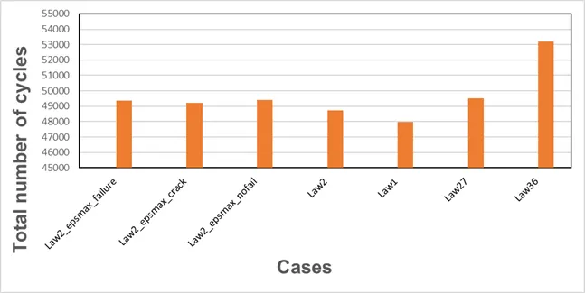
Figure -4 The comparison chart for total no. of cycles
The above graph shows that model in the case of Law36, the no. of cycles is higher than the rest.
Energy error:
The chart below illustrates the variation of error in energy in different cases.
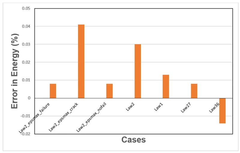
Figure -5 The comparison chart for energy error
The chart shows that the energy error is positive for all the models except Law36, which implies energy is being generated except for Law36.
Mass error
The error in mass from the table above is shown to be zero in all the cases.
Simulation time
The chart below depicts the variation of simulation time (in sec) in the different case
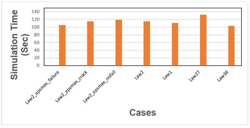
Figure -6 The comparison chart for simulation time
Energy Curve and Normal Force Curve along with Von Mises animation
CASE 1
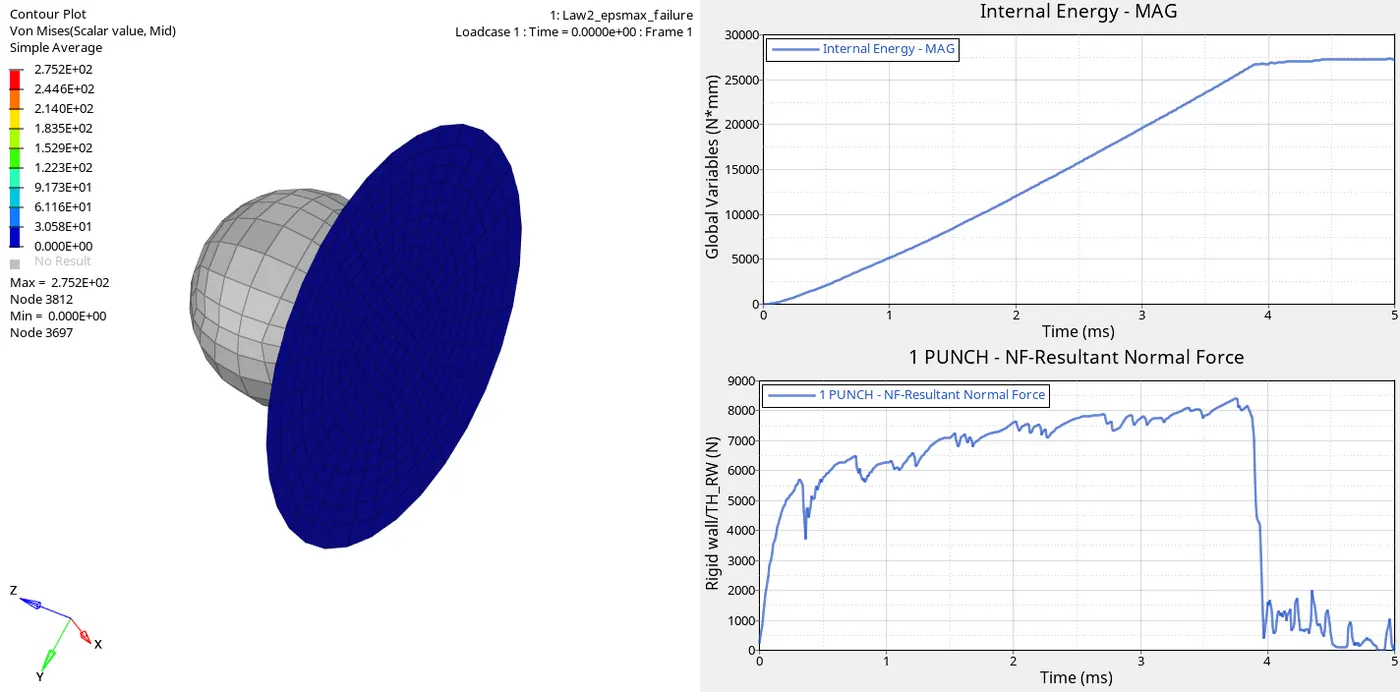
Figure -7 Case 1 LAW2_EPSMAX_FAILURE
CASE 2
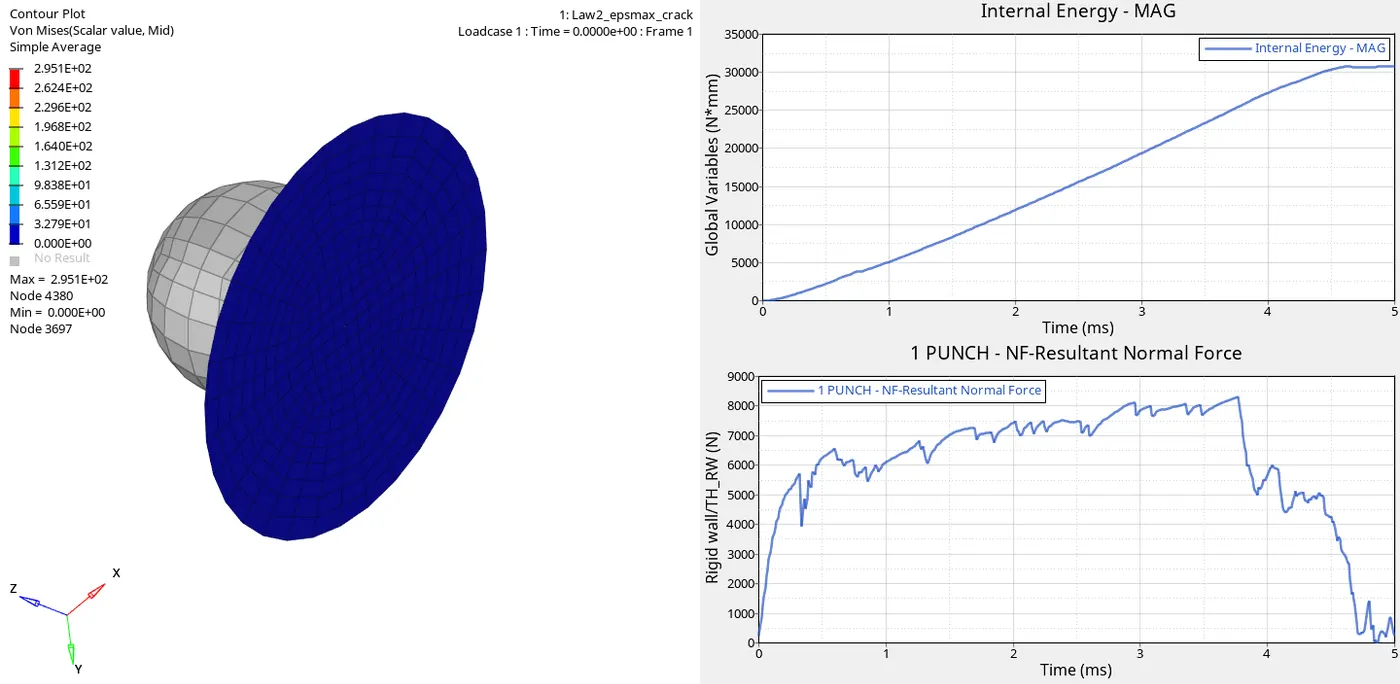
Figure -8 Case 2 LAW2_EPSMAX_CRACK
CASE 3
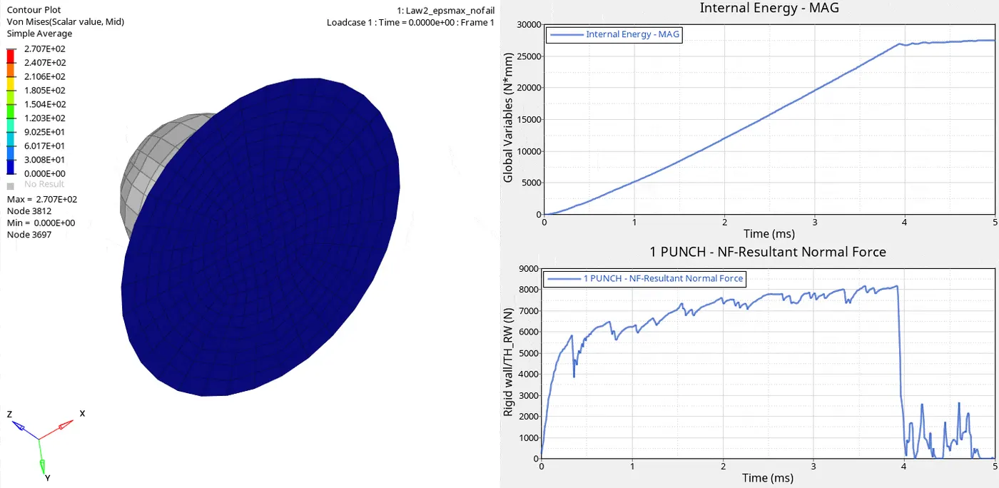
Figure -9 Case 3 LAW2_EPSMAX_NOFAIL
CASE 4
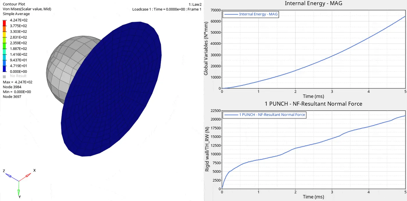
Figure -10 Case 4 LAW2
CASE 5
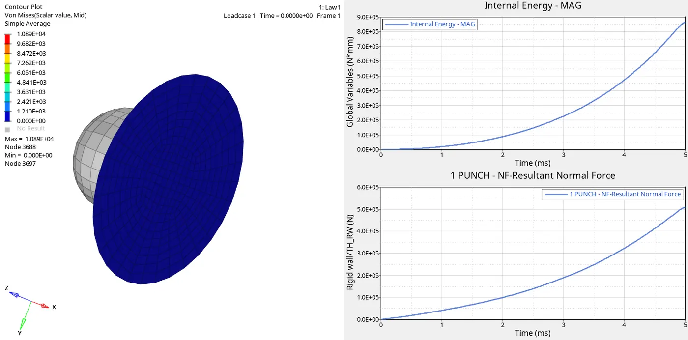
Figure -11 Case 5 LAW1
CASE 6
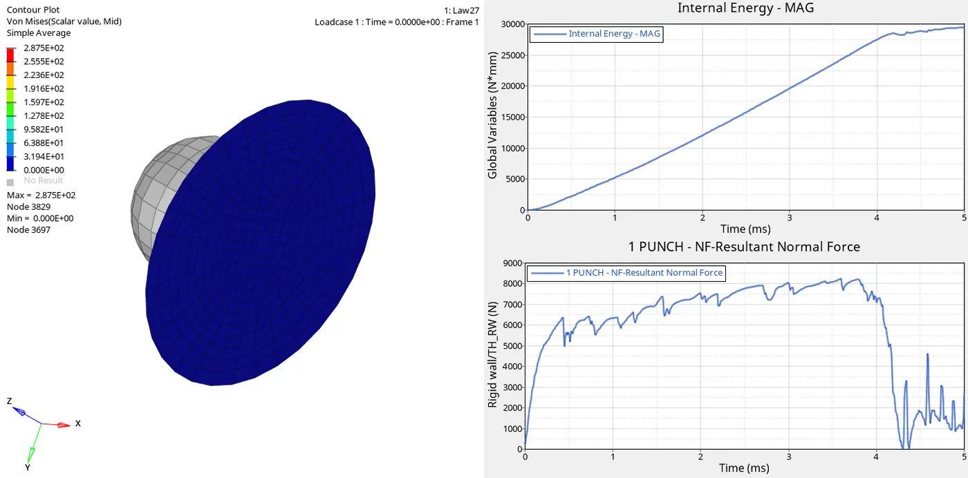
Figure -12 Case 6 LAW27
CASE 7
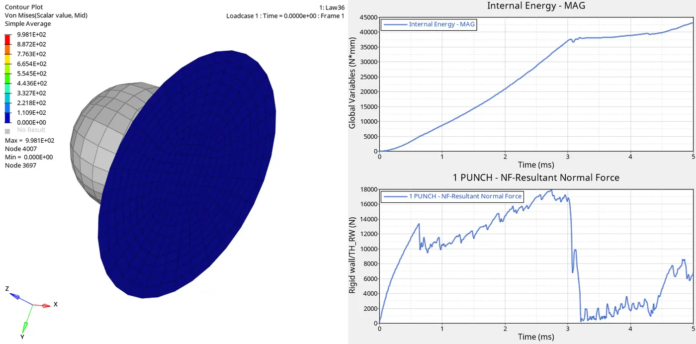
Figure -13 Case 7 LAW36
Case 1:
Isotropic elastoplastic material model using Johnson cook material and Johnson cook failure without using Ixfem, which implies no crack formation, so the elements will get deleted as shown above in Figure -7.
Case 2:
Isotropic elastoplastic material model using Johnson cook material as well as failure using Ixfem, which implies crack formation, followed by element deletion, as shown in Figure -8. Due to crack propagation, this model demonstrates the real-world scenario.
Case 3:
Isotropic elastoplastic material model using Johnson cook material but since the failure card is deleted the elements gets deleted when the plastic strain value reaches ‘eps_p_max’ value.
Case 4:
Isotropic elastoplastic material model using Johnson cook material without having ‘eps_p_max’ value, which indicates no failure in the model, as shown in Figure -10. Since the ‘eps_p_max’ value is not known, the energy will keep on increasing, which implies this model is suitable only when element failure is not under considering parameter.
Case 5:
The material model was changed to isotropic linear elastic material following Hooke’s law. No deletion of elements was observed, and the energy kept on increasing with the increase in time, as shown in Figure –11. This model is suitable for small deformation problems.
Case 6:
Isotropic elastoplastic Johnson-Cook material model with an orthotropic brittle failure model. Material damage is accounted for prior to failure. Failure and damage occur only in tension.
Case 7:
Isotropic elastoplastic Johnson-Cook material using user-defined functions for the work-hardening portion of the stress-strain curve for different strain rates. Element deletion occurs when ‘eps_p_max’ reaches a value of 0.16. It is used when the user-defined functions are known through experimental data.