Week 5 - Curve fitting

1. "popt" - It is an output of the function 'curve_fit'. It is the array that contains the optimum values of the coefficients of the cubic equation.

"pcov" - It is also an output of the function 'curve_fit'. It is a 2D array that contains the estimated covariance of the parameters in 'popt'. The diagonals provide the variance of the parameter estimate.

2. The np.array(temperature) converts the list of temperature to a numpy array since operations like "pow" are allowed on numpy arrays and not python lists.

3. "*" reference to popt / the values stored in the array popt.

4 & 6. Curve Fitting:

Linear Polynomial Curve Fitting

The python code representing the linear polynomial curve fitting is:

import numpy as np
import matplotlib.pyplot as plt
from scipy.optimize import curve_fit


# Curve fitting function
def func(t, a, b):
    return a * t + b


# Reading data file
def read_file():
    temperature = []
    cp = []
    for line in open('data', 'r'):
        values = line.split(',')
        temperature.append(float(values[0]))
        cp.append(float(values[1]))

    return [temperature, cp]


# main program
temperature, cp = read_file()
popt, pcov = curve_fit(func, temperature, cp)
fit_cp = func(np.array(temperature), *popt)

plt.plot(temperature, cp,, linewidth=3)
plt.plot(temperature, fit_cp,, linewidth=3)
plt.legend(['actual data', 'curve fit'])
plt.xlabel('Temperature[K]')
plt.ylabel('Cp')

plt.show()

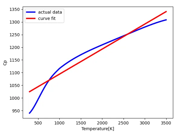
In the code above the linear curve is defined represented by "`at+b`", where the funtion is dependent on the variable t, bearing coefficients of 'a' & 'b'. Followed by the reading the data and organise the data in an array, and compare the 2 curves.

The following curve represents the output data of the curve fitting.

Cubic Polynomial Curve Fitting

The python code representing the cubic polynomial curve fitting is:

import numpy as np
import matplotlib.pyplot as plt
from scipy.optimize import curve_fit


# Curve fitting function
def func(t, a, b, c, d):
    return a * pow(t, 3) + b * pow(t, 2) + c * t + d


# Reading thermodynamic  data file
def read_file():
    temperature = []
    cp = []
    for line in open('data', 'r'):
        values = line.split(',')
        temperature.append(float(values[0]))
        cp.append(float(values[1]))

    return [temperature, cp]


# main program
temperature, cp = read_file()
popt, pcov = curve_fit(func, temperature, cp)
fit_cp = func(np.array(temperature), *popt)

plt.plot(temperature, cp,, linewidth=3)
plt.plot(temperature, fit_cp,, linewidth=3)
plt.legend(['actual data', 'curve fit'])
plt.xlabel('Temperature[K]')
plt.ylabel('Cp')

plt.show()

In the code above the cubic curve is defined represented by "`at^3 +bt^2+ct+d`", where the funtion is dependent on the variable t, bearing coefficients of 'a', 'b', 'c' & 'd'. Followed by the reading the data and organise the data in an array, and compare the 2 curves.

The following curve represents the output data of the curve fitting.

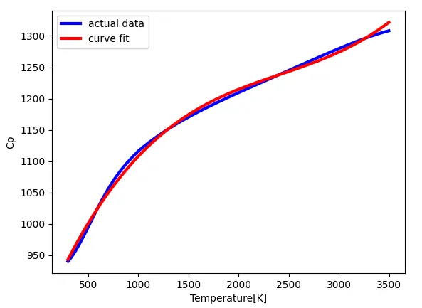
From the above 2 curves both from linear and cubic polynomial cuve fit it is evident that the cubic polynomial fits the curve more than the linear curve.

5. In order to make the curve fit more perfectly the degree of the polynomial to be fit should be increased, for example a curve of degree 4 would fit more than a curve of degree 3, and so forth. It is also inevitable that as the degree of polynomial increases the calculation complexity also increases.