Week-11 Challenge: Braking

Q1. The drive cycle used is IM240 which is inspection and maintenance driving schedule which lasts for 240 sec. It has data as follows:

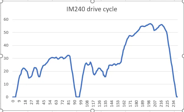
Now in order to find the braking energy needed, we will generate a matlab code.

clc;
M=1000;
t=IM240{:,1};
v=IM240{:,2};
for i=1:240
    if v(i+1)<v(i)
        E(i)=0.5*M*(v(i)-v(i+1))^2;
       
    end
end

fprintf('Total Braking energy is %d J', sum(E))
figure(1)
grid on;
subplot(2,1,1)
plot(t, v, 'linewidth', 3, 'color', 'r') 
xlabel('Time(sec)') 
ylabel('Velocity(m/s)')
title('Drive Cycle')
grid on;
hold on 
subplot(2,1,2)
plot(E, 'linewidth', 3, 'color', 'g')
xlabel('Time(s)')
ylabel('Energy(J)')
grid on;
title('Brakingnenergy')

When we run this code we get the following results-

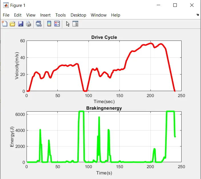
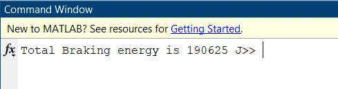
Hence the breaking energy for IM420 cycle is 190.625 kJ

---------------------------------------------------------------------------------------------------------------------------------

Q2. Why electric motor can’t develop braking torque at high speed similar to starting? How electric and mechanical brakes are coordinated?

The speed torque characteristic of an IM is given as below-

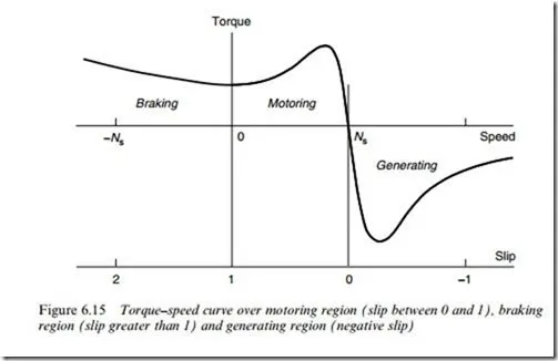
As we can see at start when speed is low, a high torque is produced but as the speed proceeds near synchronous speed, the torque becomes very less. The same applies when you brake at high speeds, the torque available is not very high and hence regenerative braking will not be very efficient.

For this reason we require mechanical brakes at high speed for effective braking.

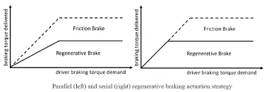
We have two types of braking that is

1. Series braking-

Where electric and mechanical brakes are used one after the other.

2. Parallel Braking:

Where both the brakes are used simultaneously.

--------------------------------------------------------------------------------------------------------------------------------------

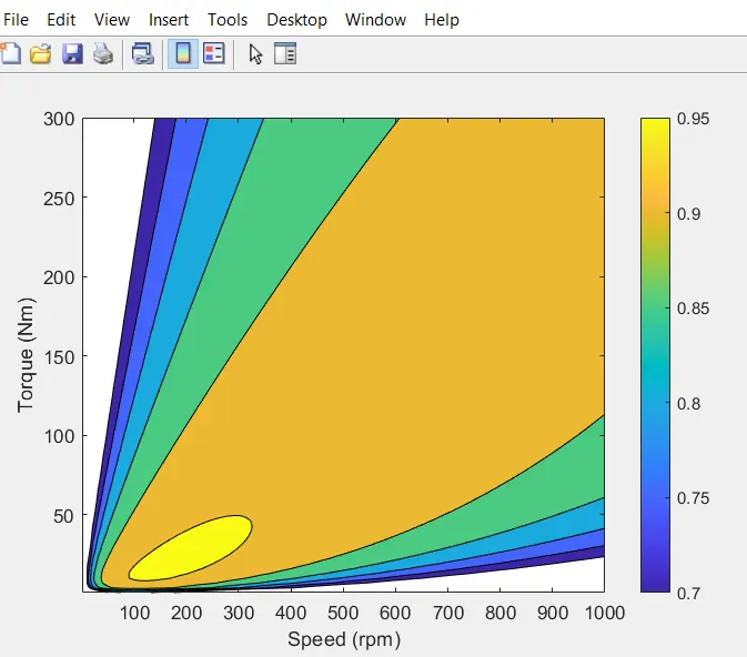
Q3. Make a MATLAB program which plots contour of given motor speed, torque and efficiency values. Attach the code as a .m file attach a screenshot of all the plots.

The following code was developed using the losses calculation equations-

Copper loss=`(K_c) tau^2`

iron loss= `K_i omega`

Windage loss= `K_w omega^3`

Constant losses C

clc;
clear all;

v=linspace(1,1000);
T=linspace(1,300);

[X,Y]=meshgrid(v,T);


kc=0.2;
ki=0.005;
kw=0.00001;
C=20;

Vo=(X.*Y);
Losses=(Y.^2)*kc+(X.*ki)+(X.^3)*kw+C;

Vi=Vo+Losses;
Efficiency=Vo./Vi;

Eff=[0.7 0.75 0.8 0.85 0.9 0.95];

contourf(v,T,Efficiency,Eff);
colorbar;
xlabel("Speed (rpm)");
ylabel("Torque (Nm)");

The plot of the above code is as follows: