Week 10: Project 1 - FULL HYDRO case set up (PFI)

Objective

we have already created a no-hydro simulation of the PFI case in the challenge "Week 9: Project 1 - Surface preparation and Boundary Flagging (PFI)", now it's time to set up a full-hydro case and see how the combustion occurs in our engine.

Engine parameters

• Engine Geometric Parameters

1. Bore =0.086 m
2. Stroke = 0.09 m
3. Connecting rod length = 0.18 m
4. RPM = 3000

• Run parameters

1. Simulation mode: Full Hydro

• Simulation time parameters

1. Start time: -480 deg
2. end time: 240 deg

• Boundary conditions

1. Piston temperature - 450K
2. Liner temperature - 450K
3. Head temperature - 450K
4. Spark Plug temperature - 550K
5. Spark Plug electrode temperature - 600K
6. Exhaust ports temperature - 500K
7. Exhaust outflow - 1 bar
8. Exhaust outflow temperature - 800k
9. Exhaust species concentration - Calculate the stoichiometric condition
10. Exhaust valve top temperature - 525K
11. Exhaust valve angle temperature - 525K
12. Exhaust valve bottom temperature - 525K
13. Intake port - 1 temperature 425K
14. Intake port - 2 temperature 425K
15. Inflow pressure - 1 bar total pressure
16. Inflow temperature - 363K
17. Inflow species - Air
18. Intake valve top temperature - 480K
19. Intake valve angle temperature - 480K
20. Intake valve bottom temeprature - 480K

• Initial conditions

Intake port - 1 (closer to combustion chamber)

• ic8h18 - 0.025508
• o2 - 0.20157
• n2 - 0.77292
• Temperature - 390k
• pressure - 1 bar

Intake port - 2 (away from combustion chamber)

• Air
• Temperature - 370K
• Pressure - 1 bar

Cylinder

• Pressure - 1.85731 bar
• Temperature - 1360K
• Stoichiometric composition

• Injection Parameters

1. Fuel flow rate = 7.5e-4 Kg/second
2. Injection start time = -480.0
3. Injection duration = 191.2
4. Fuel temperature = 330K

• Nozzle positions

Nozzle diameter = 250 micro-meter

Circular injection radius = Nozzle radius

Spray cone angle = 10

• Nozzle 0
  • center 0.0823357 0.00100001 0.07019
  • Align Vector -0.732501 0.210489 -0.647408
• Nozzle 1
  • center 0.0823357 -0.00099999 0.07019
  • Align Vector -0.732501 -0.210489 -0.647408
• Nozzle 2
  • center 0.0823357 -0.0004 0.07019
  • Align Vector -0.5 -0.2 -0.647408
• Nozzle 3
  • center 0.0823357 0.0003 0.07019
  • Align Vector -0.5 0.2 -0.647408

Spark Ignition Parameters

• Start of spark = -15 deg
• Spark duration = 10 deg
• Spark location = -0.003 0 0.0091
• Spark radius = 0.0005m

Physical models

• spray modelling

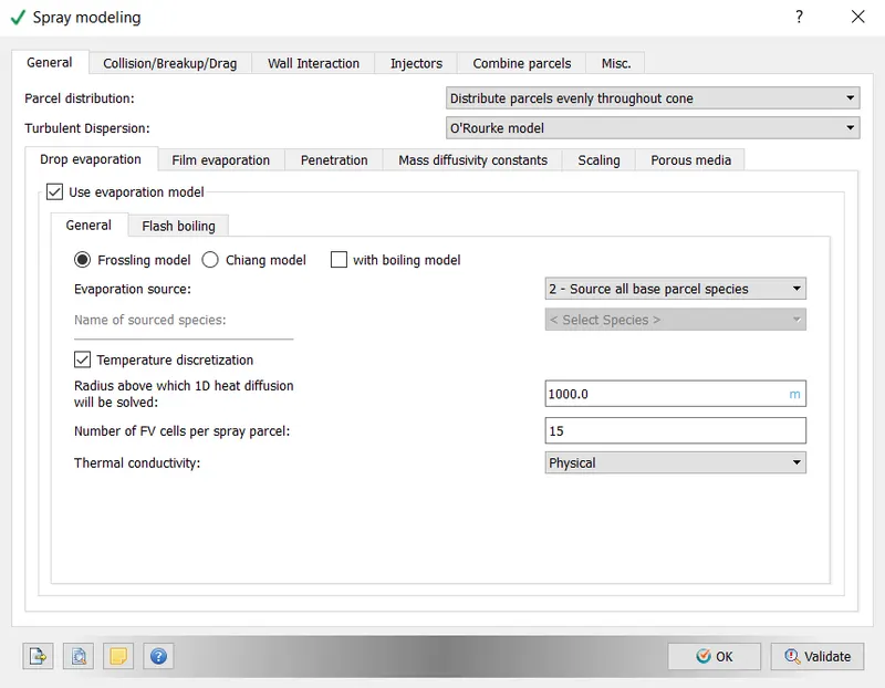
Figure 1

In Figure 1 we choose parcel distribution to be distributed evenly throughout the cone. In spray modelling, turbulent dispersion is an important concept, as the spray will be injected in the high-velocity flow of air which will be turbulent, it will affect the atomization and mixing process of fuel, therefore the process should be predicted properly using the "O'Rourke model". In addition In temperature discretization, we choose the fuel parcel radius to be 1000m, reason for this nonintuitive decision at first glance is that above that value solver will be considering that within the fuel parcel volume temperature gradient will be present and will solve ODEs for every parcel, which will be time-consuming, therefore as we don't have experimental data we don't use appropriate value for the parcel radius to cut the computational time an get a bit less accurate results.

Figure 2

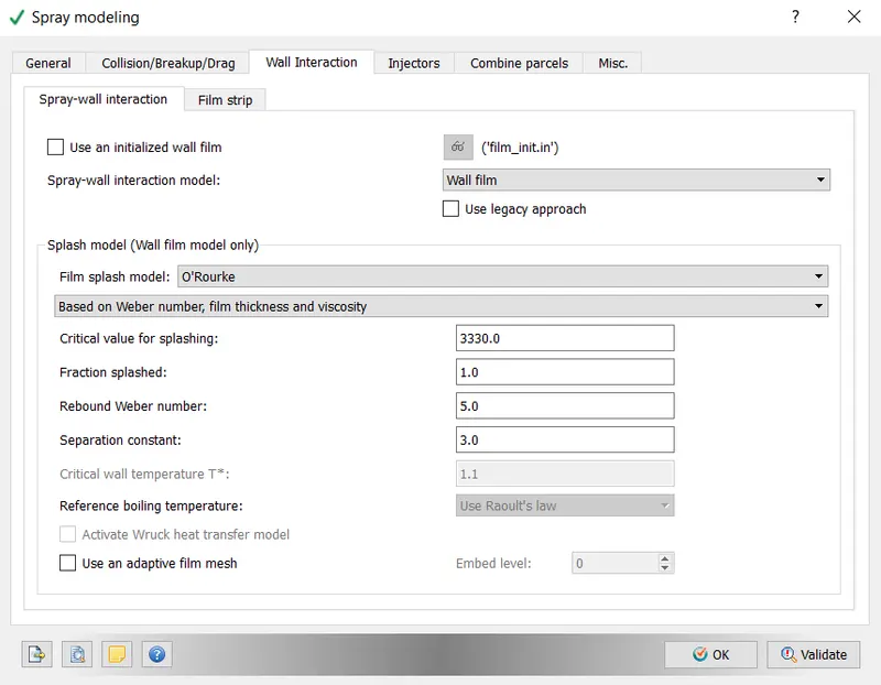
Figure 3

In the wall interaction section, we predict spray-wall interaction using the "wall film" model. Film splash will be calculated using the "O'Rourke" model, which will be based on the Weber number. The Weber number (We) is a dimensionless number in fluid mechanics that is often useful in analysing fluid flows where there is an interface between two different fluids, especially for multiphase with strongly curved surfaces. It can be thought of as a measure of the relative importance of the fluid's inertia compared to its surface tension, meaning this number is used to predict when the fuel parcel will break up into smaller parcels before it vaporizes and will be transformed into a gas phase.

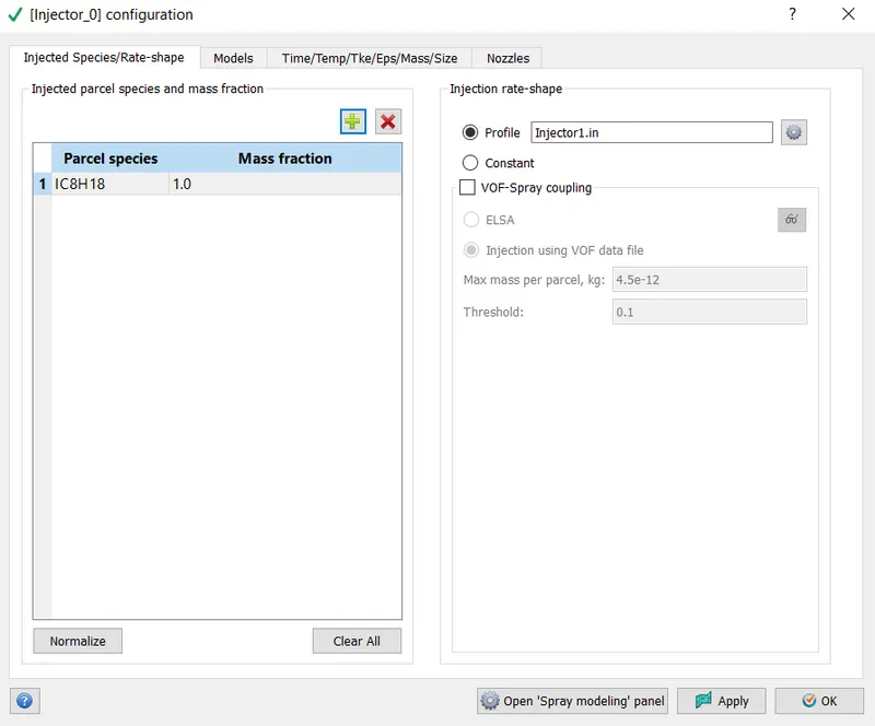
Figure 4

As shown in Figure 4 as a fuel we are using C8H18 with a mass fraction of 1.

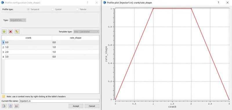
Figure 5

In Figure 5 profile of the injector is shown. As you see we have fully developed injection throughout the injection phase. Which lasts from the crank angle of -480 to the crank angle of 288.8, shown in Figure 6 below.

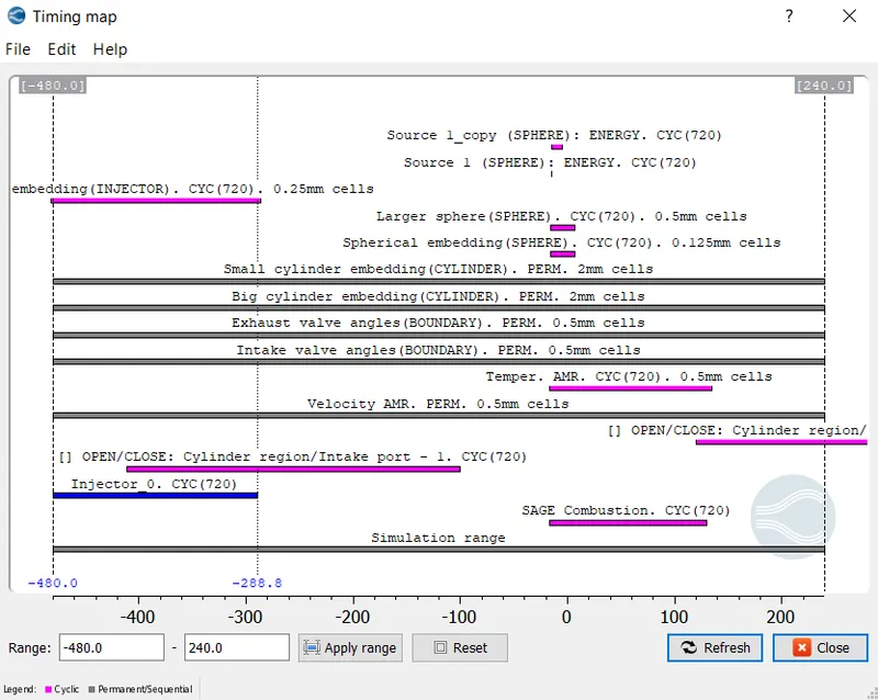
Figure 6

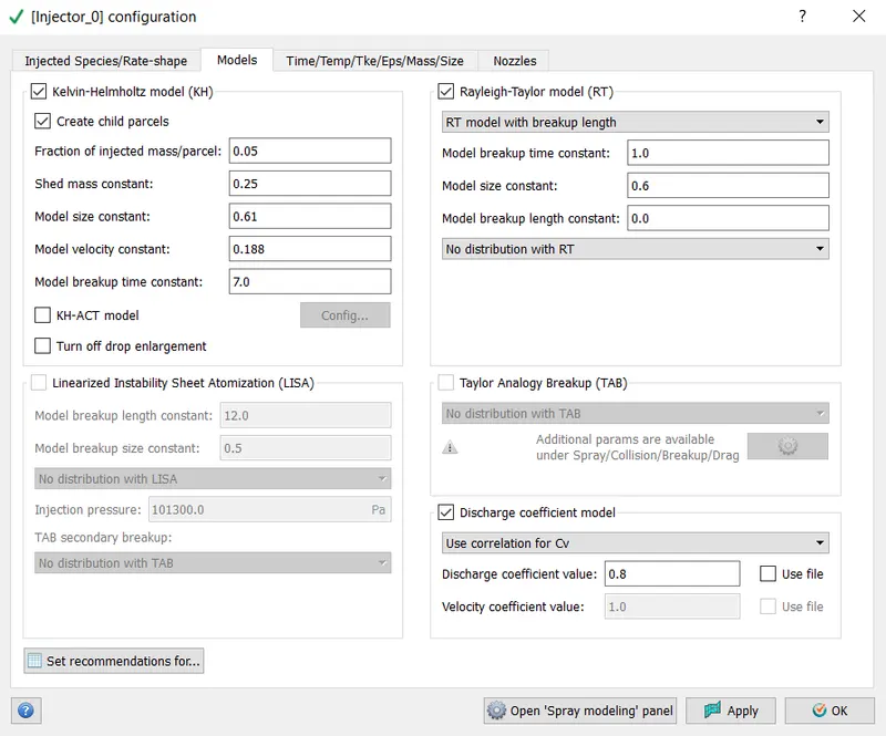
Figure 7

Mathematical models used for spray modelling are shown in Figure 7. KH & RT models are most applicable for the cases we intend to simulate.

Note: All the coefficients in the above-mentioned models are set as a recommended values.

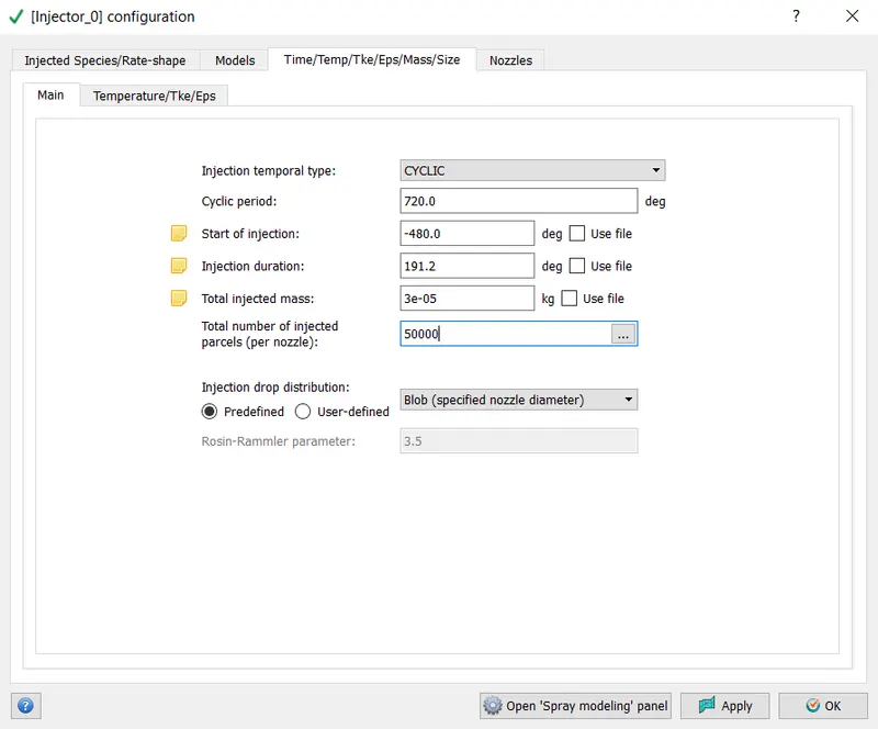
Figure 8

In Figure 8 injection period is specified, moreover, as we saw in the input values of the simulation fuel flow rate is 7.5e-4 Kg/second but in the Total injected mass we set 3e-05kg in other words 3 micrograms, as it's calculated per the duration of the injection time in our case.

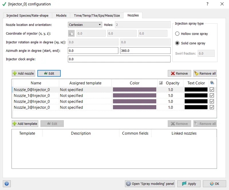
Figure 9

In Figure 9 four injector nozzles are introduced. Nozzle geometrical and orientation parameters are already given in the "Engine parameters" chapter above, however in Figure 10 one of the four nozzles will be shown.

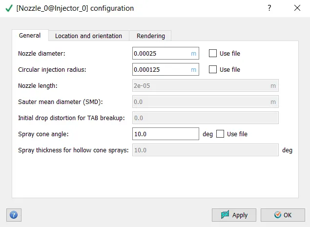
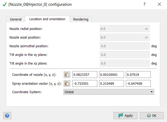
Figure 10

• Combustion Modelling

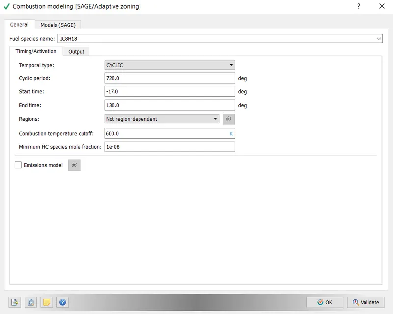
Figure 11

In Figure 11 Combustion process time is shown using the crank angle. As we see combustion process will be calculated during the period of crank angle of -17degrees to 130degrees.

As a combustion model, we are using the so-called "SAGE" model which is the most suitable for gasoline engine applications.

• Turbulence model

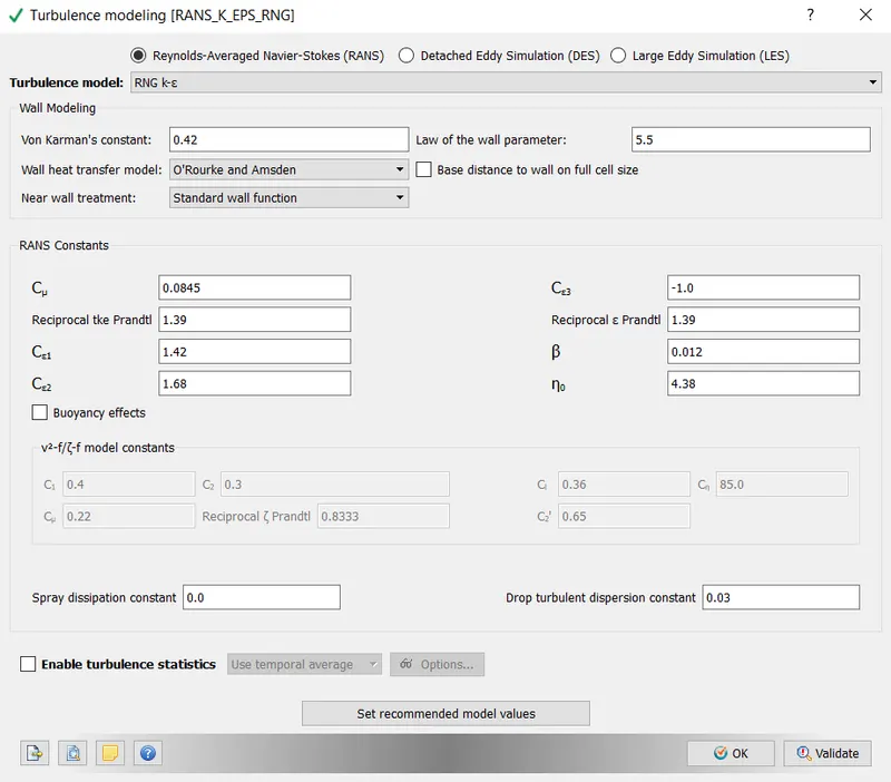
Figure 12

• Source/Sink modelling

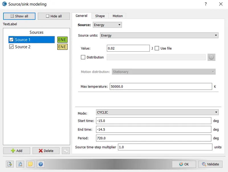
Figure 13

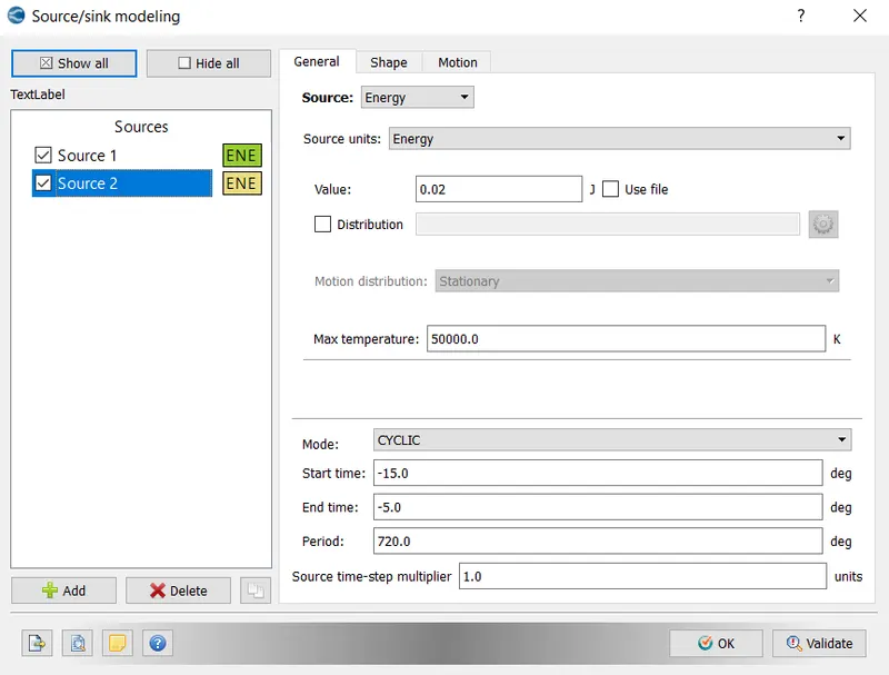
Figure 14

In Figures 13 and 14 spark plug parameters are shown. As you see, we have two sources: the first one in Figure 13 source1 is the energy source of 20mj active only about the half crank angle, from -15degrees to -14.5degrees and the source2 in Figure 14 provides the same amount of energy, however, the active period is larger, from -15degrees to -5 degrees. All of this configuration is caused by spark plug three phases: breakdown, arc discharge, and glow discharge. Initially, we need more energy to occur proper conduction between a spark plug gap, therefore we add up the energy of those two sources and get 40mjs from -15degrees of crank angle to -14.5degrees, afterwards less energy is needed to maintain conduction therefore the provided energy is reduced from 40mjs to 20mjs from the crank angle of -14.5degrees to -5degrees.

Mesh

• base grid size

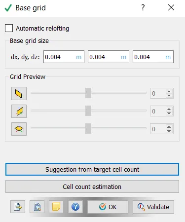
Figure 15

• Fixed embedding

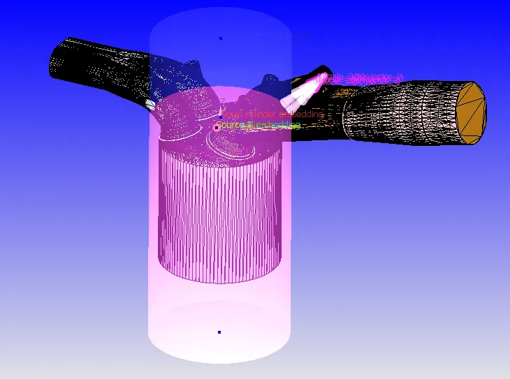
Figure 16

In Figure 16 all the transparent objects within the engine geometry are fixed embedding, which will be discussed using the next Figures.

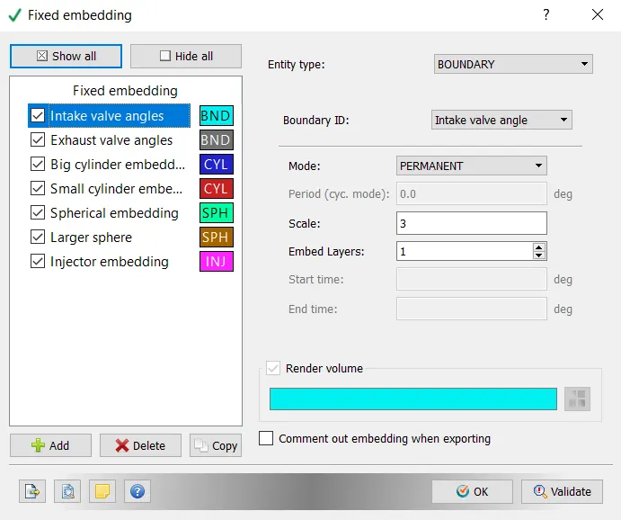
Figure 17

Within the entire model, we have several concerning areas where the mesh should be more accurate than the base grid size to adequately predict the ongoing process.

The first two embeddings are located at the intake and exhaust valve angles, at those locations mesh will be refined with the scale of 3, meaning the base grid size which is 4mm will be divided into 8, as the embedding scale is 3 `embedded grid size = (base grid size)/(2^n)` where - n is the scale, therefore our mesh size will be 0.5mm in those locations.

The third and fourth embeddings are big transparent cylinders shown in pink colour in Figure 16, which are used to refine the mesh throughout the cylinder region, where all 4 strokes of the engine will occur.

The fifth and sixth embeddings are used in the spark plug location to appropriately operate the adaptive mesh refinement (AMR) in that location. When the spark plug ignites we encounter an instantaneous rise in temperature of mixed fluid, therefore we have significant curvatures in the second-order derivatives of temperature, as the grid size is not too fine at the spark plug location we consider that AMR will no longer act in that location properly, that's why we refine the mesh at the spark plug location 1degree of crank angle before the spark plug ignites.

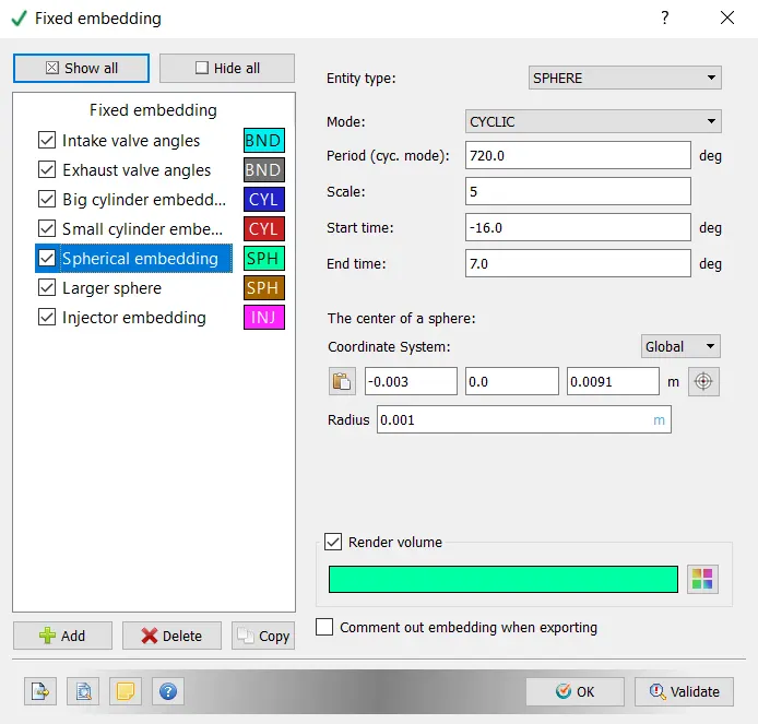
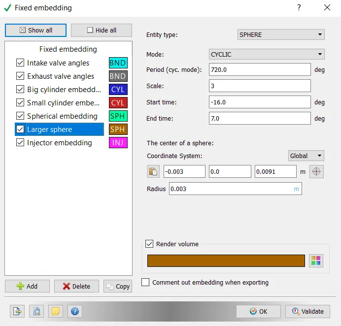
Figure 18

To visualize what we are talking about the link is provided below to show the animation of mesh generation within the spark plug location.

Figure 19

The same is done at the location of fuel injectors to provide refined mesh for AMR properly acting on velocity curvatures during the injection phase, please see Figure 20.

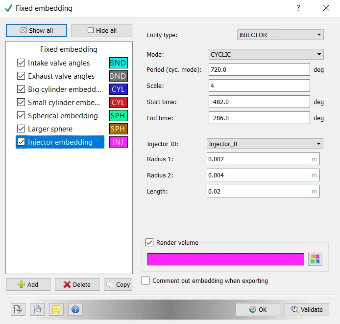
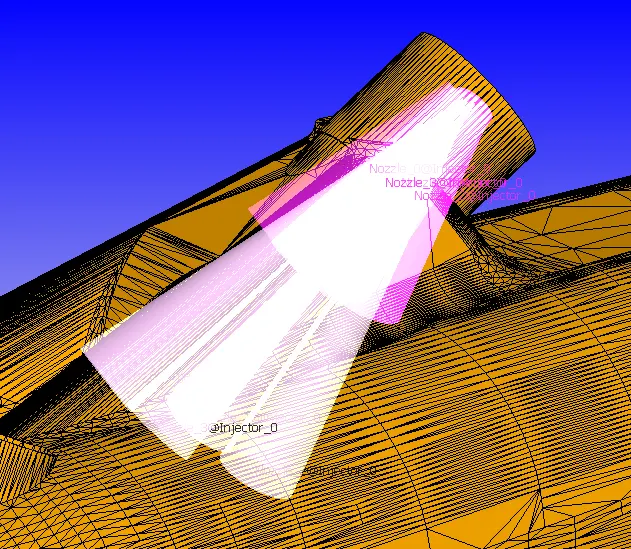
Figure 20

Note: In Figure 20 injector fixed embedding is shown in pink colour.

• Adaptive mesh refinement

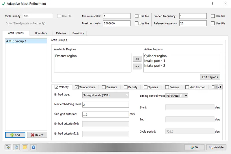
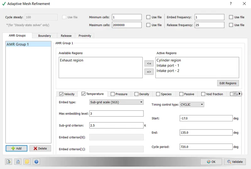
Figure 21

Post Processing

• Compression ratio

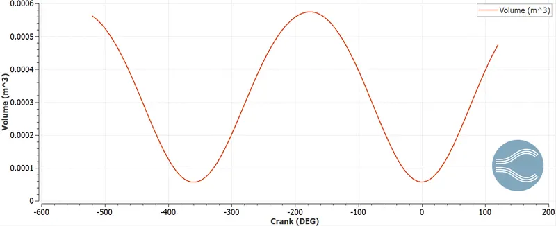
Figure 22

From Figure 22 we can find out what is the maximum and minimum values of the volume to determine the compression ratio. It turns out the maximum volume to be 5.74e-4 and the minimum volume 5.70e-5, therefore the compression ratio is `(5.74e^-4)/(5.70e^-5) = 10.07`.

• Why do we need a wall heat transfer model?

While designing internal combustion engines it's crucial to properly predict heat transfer between fluid and the walls the fluid is interacting with to find out how the dimensions of the engine parts will change, Furthermore heat transfer prediction will also be used while designing engine cooling systems. To adequately predict thermal interaction between hot fluid and wall surfaces, we need dedicated heat transfer models.

• Combustion efficiency of the engine

Combustion efficiency represents how effectively the fuel energy was released during the combustion process. In real engines, fuel is never burnt completely, that's why we have as an exhaust product unburnt substances like carbon monoxide CO, nitrogen monoxide `NO_x` or unburnt hydrocarbons HC.

Combustion efficiency `eta_c` is defined as a ratio of the energy released during the combustion and the theoretical energy of the fuel.

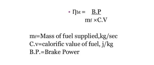
Figure 23

In Figure 23 combustion efficiency equation is provided. Using this equation we can determine combustion efficiency in our case.

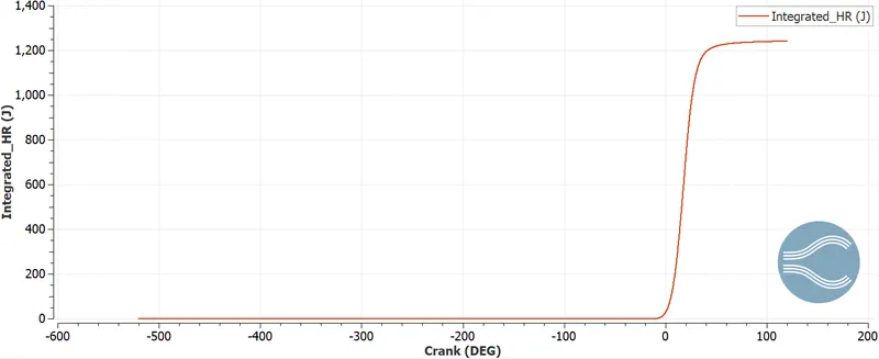
Figure 24

In Figure 24 integrated heat release is shown, which provides information about how much energy was released by the fuel during the combustion process.

The calorific value of the fuel in our case is 44000kj/kg and the mass of the fuel-injected per full cycle is 3e-5kg, 3 micrograms.

`eta_c= 1.24/(44000*3e^-5) = 0.939~~94%`.

According to the equation above combustion efficiency in our case is 94%.

• The engine performance calculator

In "Converge CFD" there is a useful tool called "Engine performance calculator" which provides engine performance data using Thermo.out file.

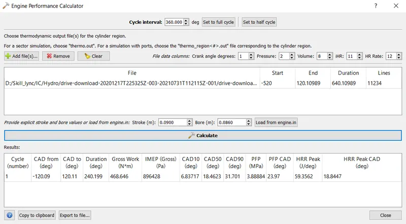
Figure 25

From the calculator, we can determine engine power and torque. As you see, work done is "Gross Work (N*m)" which is 468.646Nm. The duration of the process is 240.199degrees, the rotational velocity of the engine is 3000RPM, therefore rotation per second is `3000/60=50`. The total degree is `50*360=18000`, thus the time taken by the cycle is `240.199/18000=0.01334`, therefore power is Gross work divided by the time `468.646/0.01334=35130.884KJ=35.13KW`.

The torque `T = (Power*60)/(2*pi*N) = (35130*60)/(2*3.14*3000)=111.878Nm`

• What is the significance of ca10, ca50 and ca90?

ca10, ca50 and ca90 represent at what crank angle 10, 50 and 90 per cent of fuel is burnt. We can determine those values using the "Engine performance calculator" shown in Figure 25.

The physical significance of CA10 is that it is used to identify the start of ignition in a diesel engine, whereas the CA50 indicates the end of premixed combustion and the start of diffusion combustion of fuel used in the engine.

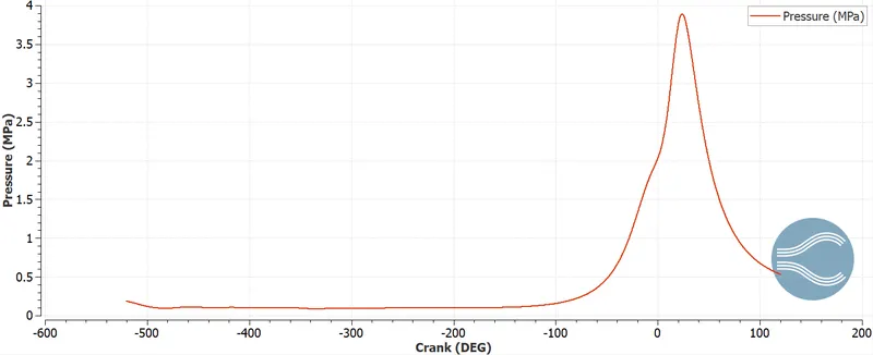
Figure 26

In Figure 26 we see how pressure changes inside the cylinder throughout the complete process, according to Figure 26 we can easily determine the peak pressure of the combustion chamber which is approximately 3.88MPa, in other words, 38.8Bar.

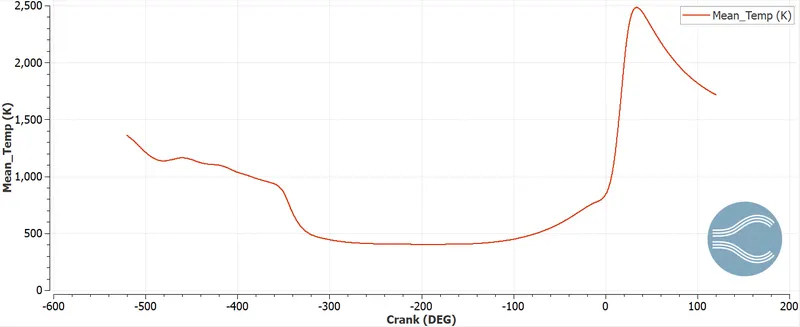
Figure 27

• Emissions

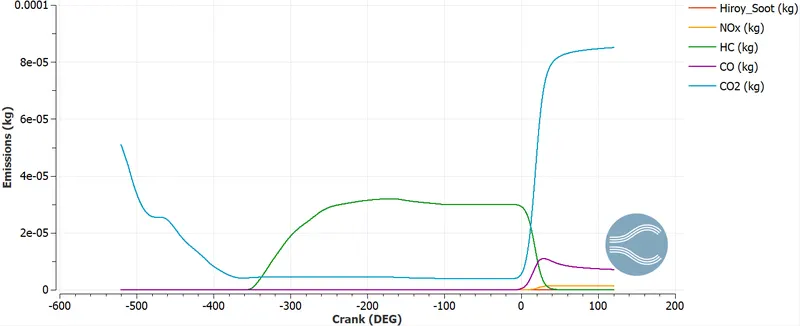
Figure 28

According to Figure 28, the amount of emission gases can be determined, which is imperative while designing an IC engine.

• Animations

Fuel spray generation

Figure 29

Combustion temperature animation

Figure 30

Combustion velocity animation

Figure 31

Combustion pressure animation

Figure 32

Section-Cut. Combustion temperature animation

Figure 33

Section-Cut. Combustion velocity animation

Figure 34

Conclusion

We successfully simulated the PFI case. Created complete set-up of Full-Hydro case of the engine. post-processed the simulation results and determined engine power and torque.