Ahmed Body Challenge

Objective

Answer the following questions

• Describe Ahmed body and it's importance
• Explain the reason for the negative pressure in the wake region.
• Explain the significance of the point of separation.

Expected results

• Velocity and pressure contours.
• The drag coefficient plot for a refined case. ( For velocity of 25m/sec, the drag coefficient should be around 0.33).
• The vector plot clearly showing the wake region.
• Perform the grid independency test and provide the values of drag and lift with each case.

Ahmed body and it's importance

The Ahmed body is a generic car body, in other words, simplified vehicle model. The airflow around the ahmed body captures the essesntial flow features an automobile. It has very simple shape, however allows us to capture characteristic features which helps us to design automobile shapes.

This model is also used to describe turbulent flow around a car-like geometries. Once the numerical model is validated, it's used to design new models of an automobile.

Geometry

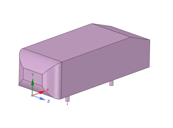
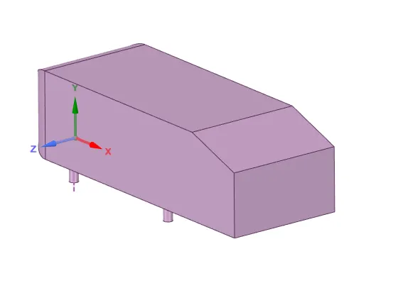
Figure 1: Ahmed body front and rear (Isometric views)

• Virtual Wind tunnel using SpaceClaim

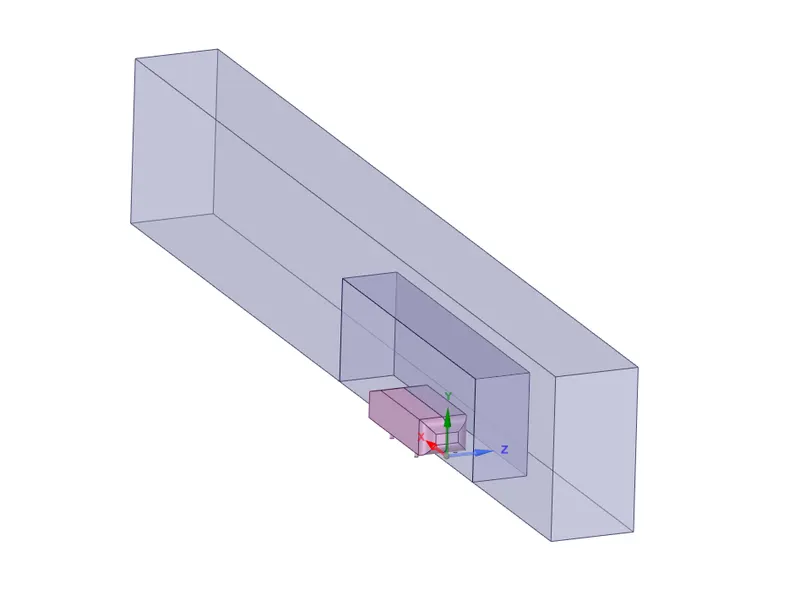
Figure 2: Ahmed body and Wind Tunnel (Half-Cut)

As you see in The Figure 2 we create 2 enclosures in order to create domain around the study object "Ahmed body".

We cut the fluid doamin in half because as the Ahmed body is symmetrical object we can rely on only the half of the fluid zone in order to decrease the computational cost of the simulation.

• Wind Tunnel geometrical dimensions

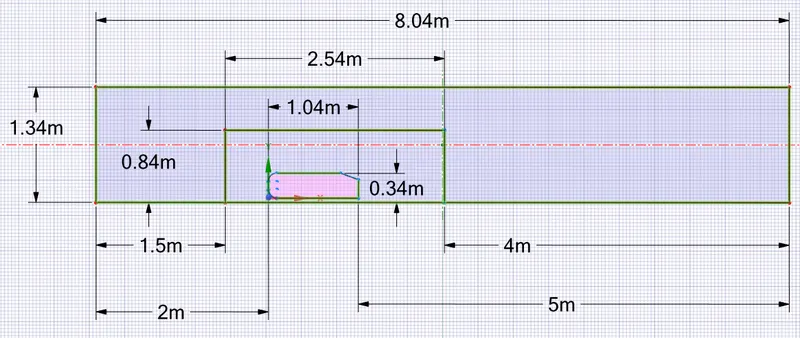
Figure 3: Wind Tunnel (Side view)

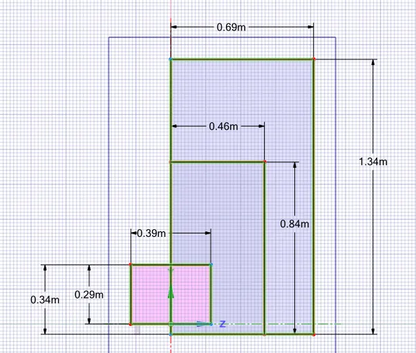
Figure 4: Wind Tunnel (Front view)

Mesh Generation

As we already described the whole fluid zone is divided into 2 parts (Enclosures).

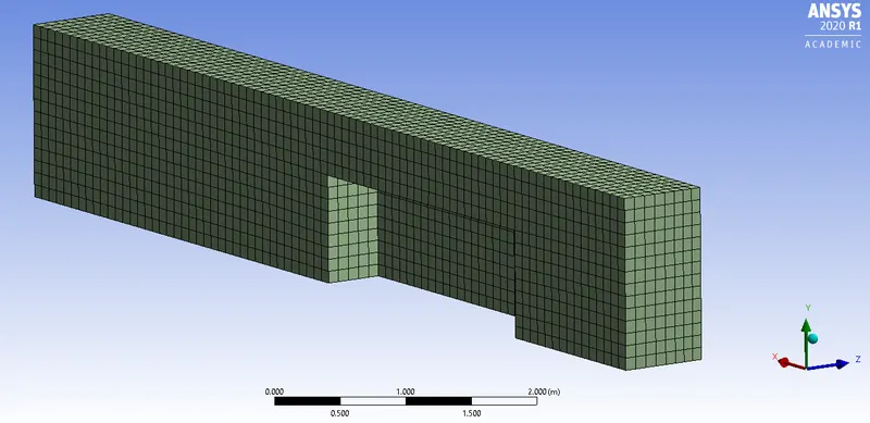
Figure 5: Enclosure 1

As we see in the Figure 5 we use Multizone method to generate hexa type mesh elements for the Enclosure 1. For CFD as we know Tetra mesh is more relevant, however we consider that the domain shown in the Figure 5 does not need Tetra type or a small value of a mesh element size because airflow will be laminar. Element size for the Enclosure 1 is 0.1m.

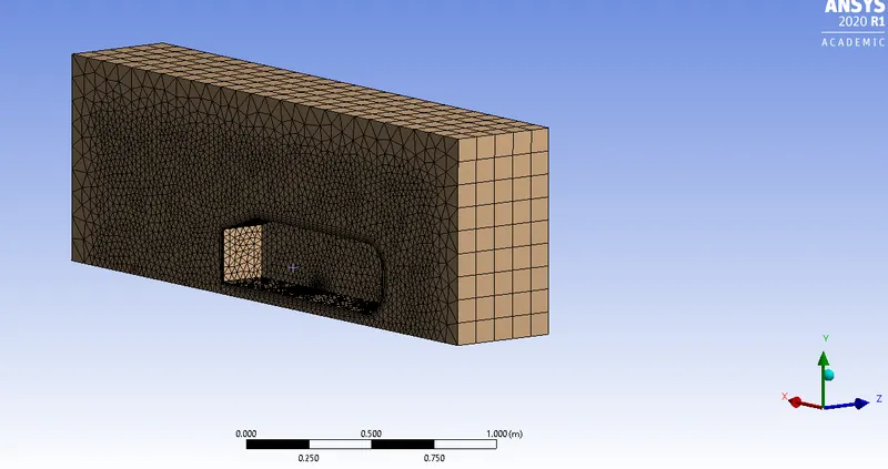
Figure 6: Enclosure 2

In the Figure 6 the fluid domain is an Enclosure of the Ahmed body where the airflow structure will not be laminar. As the flow passes around the object we may excpect flow separations and wake regions behind the Ahmed body, The Enclosure 2 is the place where the turbulence flow will be precent, therefore we generate much finer Tetra mesh than in The Enclosure 1 shown in the Figure 5. Mesh element size for the Enclosure 2 is 0.03m.

The msot important thing while generating computational mesh is to optimally set the mesh element size values in order to get the results with the desired tolerance, furthermore computational cost must be as least as possible, Therefore we are using Y+ boundary layer concept to find out the size of the first layer of the mesh at the surface of the Ahmed body.

For Turbulent layer capturing we will need the Y+ value to be in the following range: 50<Y+<300.

Firstly, we will have Y+ with the value of 300. To calculate the first layer mesh element size we use the website: https://www.pointwise.com/yplus/

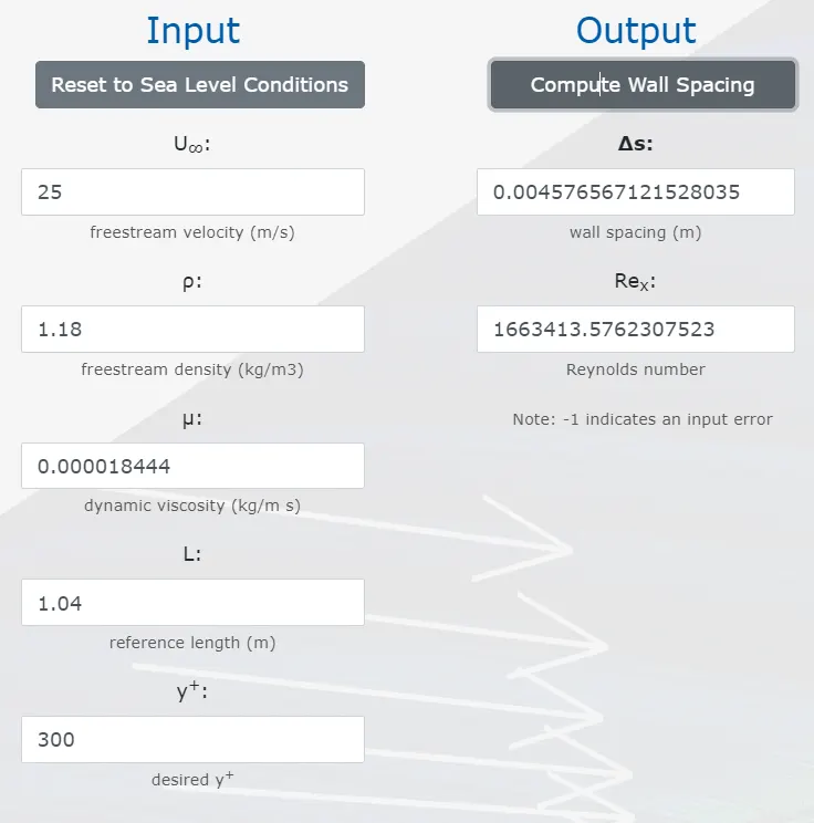
Figure 7: Y+ 300

As you see in the Figure 7 size of the first layer element should be 0.00457m in order to get the Y+ value of 300 at the Ahmed body surface.

Note: In the figure 7 all the input values correspond our case. Velocity inlet is 25m/s. Air density is 1.18`(kg)/m^3` as the air temperature is 300K and the Characteristic length of the Ahmed body is 1.04m as shown in the figure 3.

We use inflation layer method to generate proper grid with the provided mesh element size.

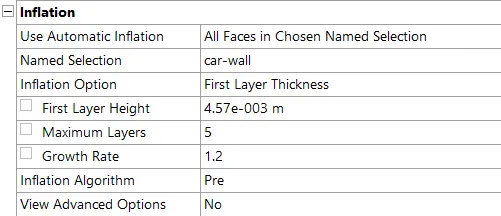
Figure 8: Inflation layer

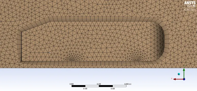
Figure 9: Inflation layer visualization

• Mesh quality and statistics.

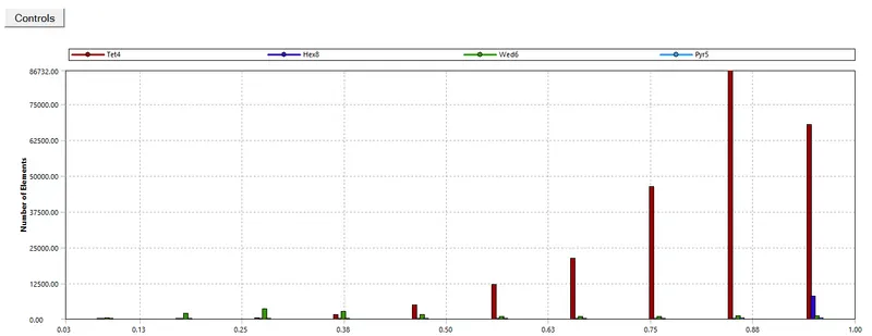
Figure 10: Element Quality

To identify the quality of the mesh as a mesh metric we are using "Element Quality".

Figure 11: Statistics

• Named Selection of the Boundaries

Inlet

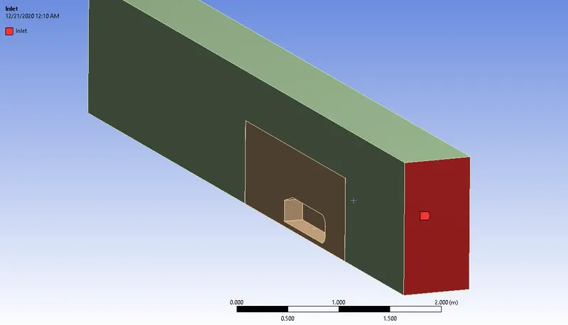
Figure 12: Inlet

Outlet

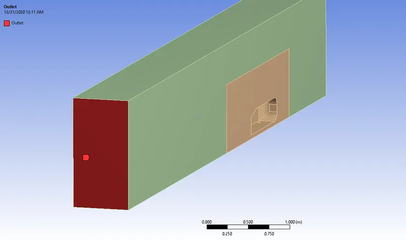
Figure 13: Outlet

Symmetry 1 & 2

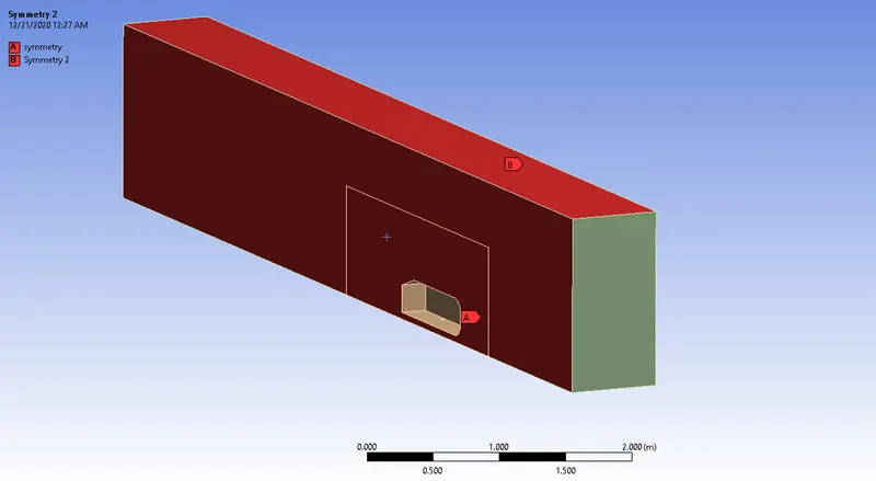
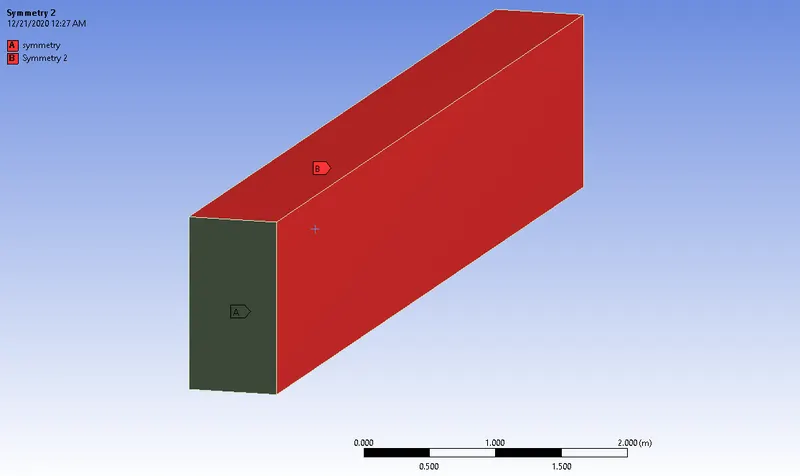
Figure 13: Symmetry

car-wall

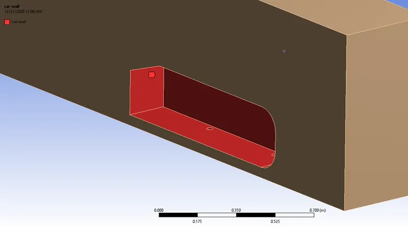
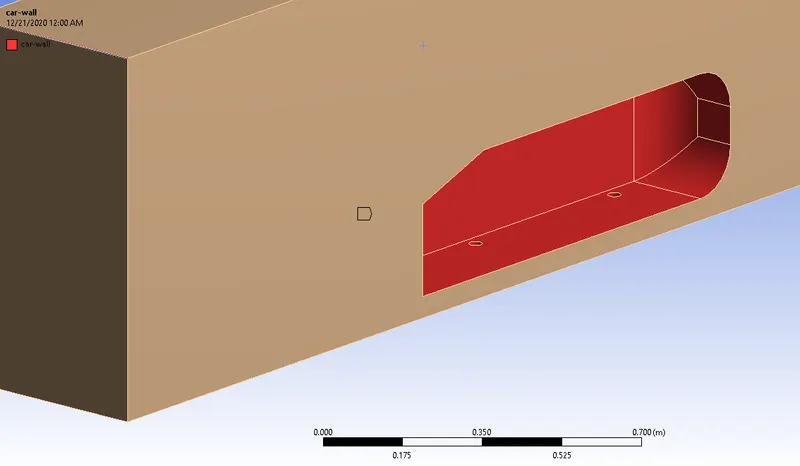
Figure 14: car-wall

Ground Wall

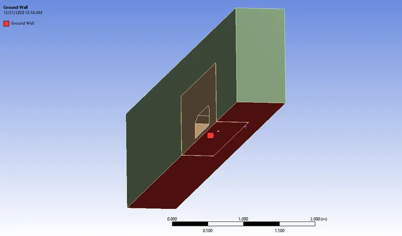
Figure 15: Ground Wall

Case Setup

We are running a steady state simulation, capture lift and drag coefficients, Furthermore we intend to capture the wake region behind the Ahmed body in order to investigate why the flow is separated and why we have negative pressure zone in the wake region.

As a turbulent solver we are using `k-omega` SST model in order to correctly capture flow separation and wake region in our study.

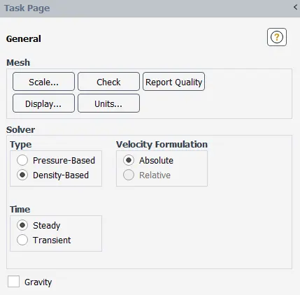
Figure 16: General

Fluid (Air ideal gas)

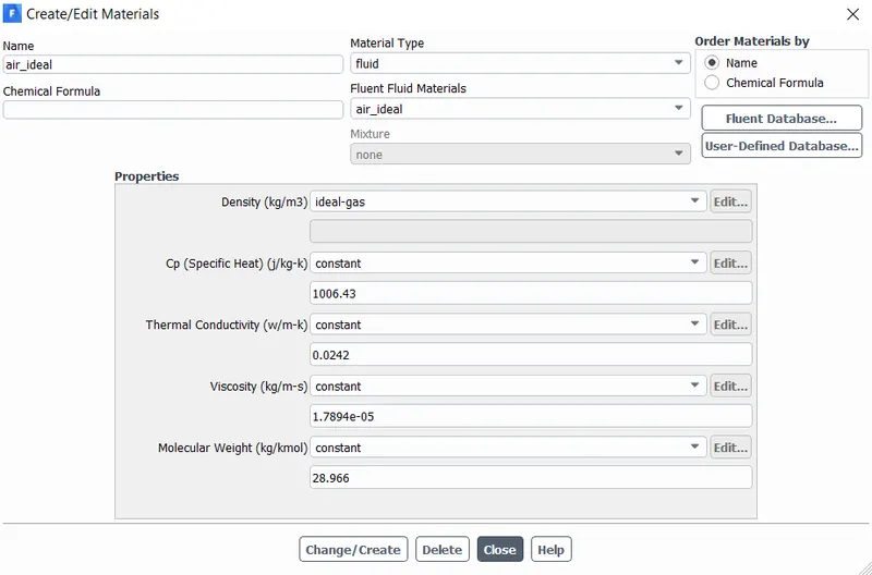
Figure 17: Air ideal gas

• Boundary Conditions

Inlet

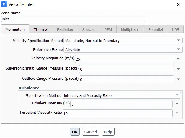
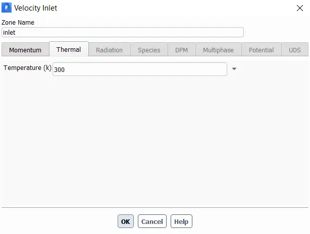
Figure 18: Velocity Inlet

Outlet

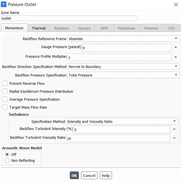
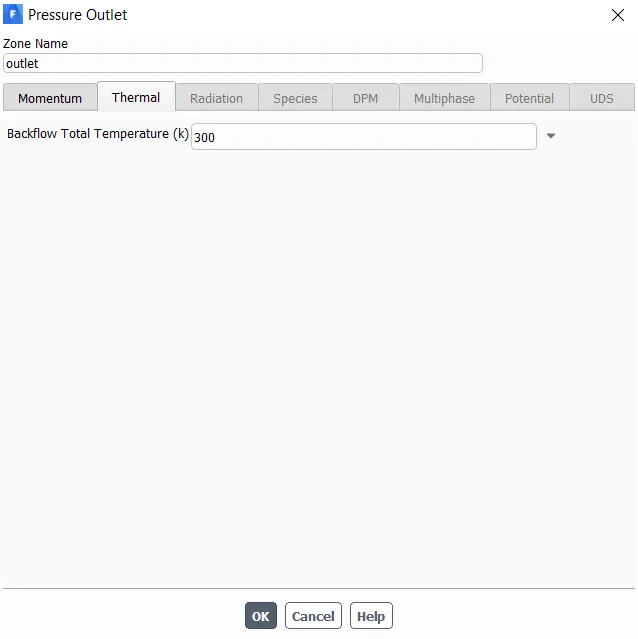
Figure 19: Pressure Outlet

car-wall

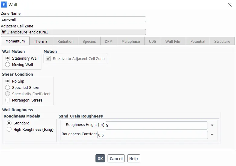
Figure 20: car-wall

all other named selection faces are symmetrical boundary conditions, as we already discussed that the whole domain is cut in half in order to reduse computational time we need to set some faces as a symmetric ones, however "Ground Wall" shown in the Figure 15 is also a symmetric boundary, due to the boundary layer phenomenon. As you see in the Figure 20 "car-wall" boundary is a fixed wall with "No slip" shear condition, meaning boundary layer will be present on the car-wall surface. As we are simulating car-like shape object aerodynamics we should not rule out that in real life when the automobile is moving boundary layer will not be present on the ground, if we set that face as a fixed wall with the "No slip" condition it may give us errors, therefore "Grounf Wall" is set to be a symmetry in order to eliminate boundary layer creation.

• Results

Scaled Residuals

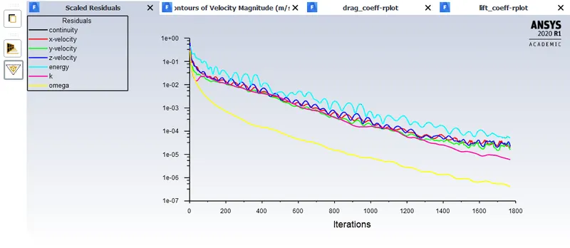
Figure 21: Scaled Residuals

• Drag coefficient

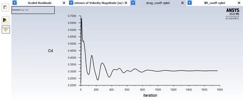
Figure 22: Drag coefficient

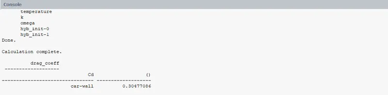
Figure 23: Drag coefficient Compute

As we see the Drag coefficinet appeared to be 0.30477. According to the experimental data it should be 0.33.

Results accuracy is approximately 92 percents which is acceptable, however we intend to continue mesh independent study to figure out if further mesh refinement with the lower value of Y+ will help to reach experimental value as close as possible.

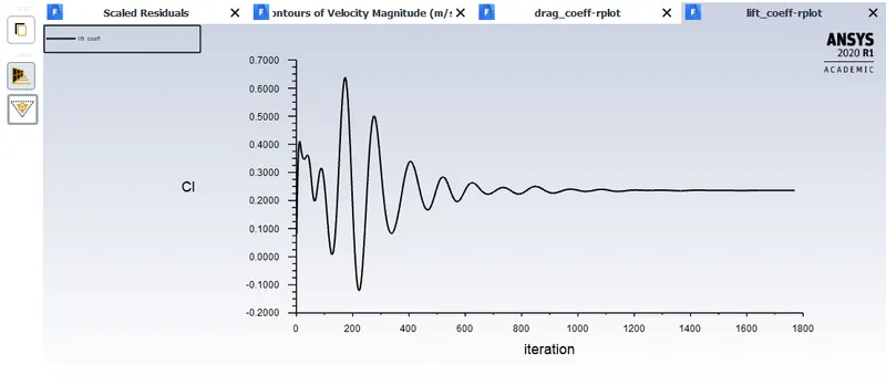
Figure 24: Lift coefficient

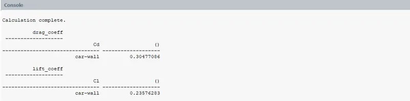
Figure 25: Lift coefficient Compute

The lift coefficinet appears to be 0.2357.

Mesh refinemet Y+ 150

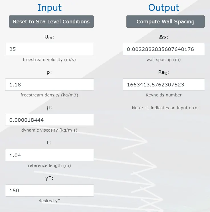
Figure 26: Y+ 150

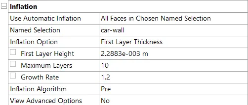
Figure 27: Inflation layer

As you see in the Figure 27 we set the first alement size as it was calculating using the website: https://www.pointwise.com/yplus/.

Inflation layer were increased up to 10.

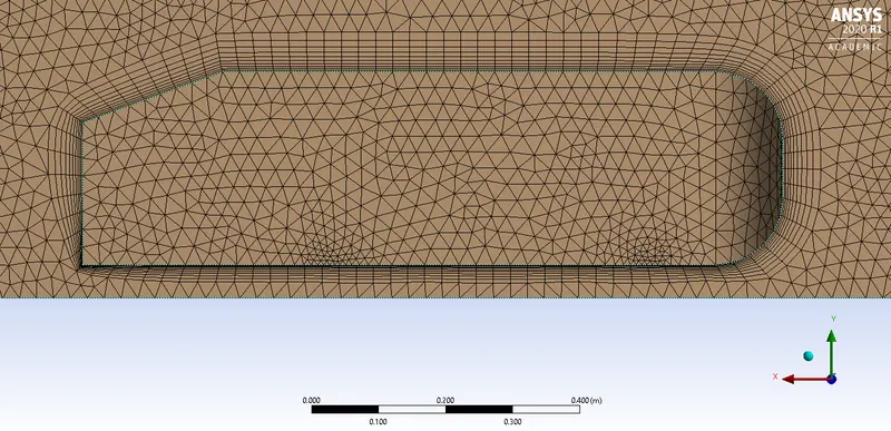
Figure 28: Inflation layer visualization

• Mesh quality and Statistics

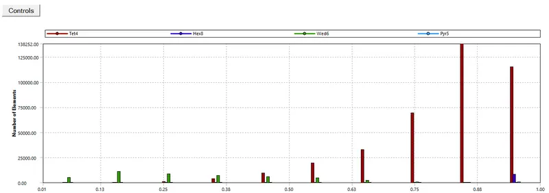
Figure 29: Mesh Quality

Figure 30: Statistics

• Results

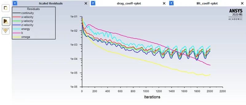
Figure 30: Scaled Residuals

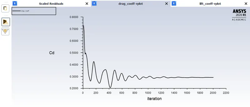
Figure 31: Drag coefficient

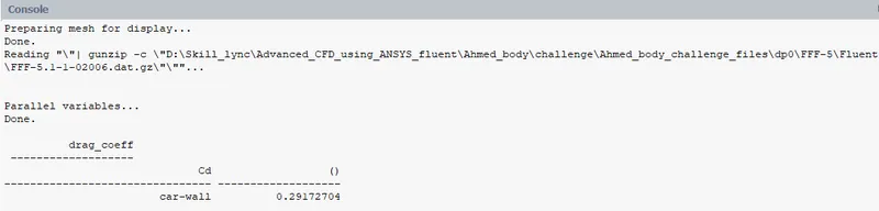
Figure 32: Drag coefficient compute

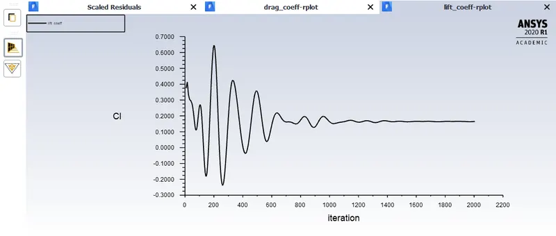
Figure 33: Lift coefficient

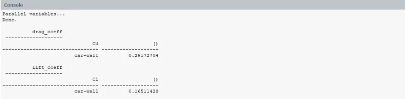
Figure 34: Lift coefficient compute

Mesh refinemet Y+ 50

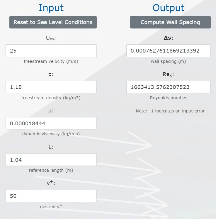
Figure 35: Y+ 50

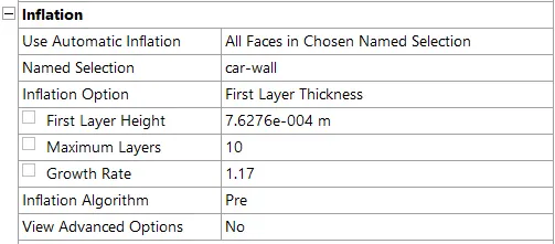
Figure 36: Inflation layer Y+ 50

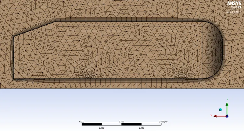
Figure 37: Inflation layer visualization

• Mesh quality and Statistics

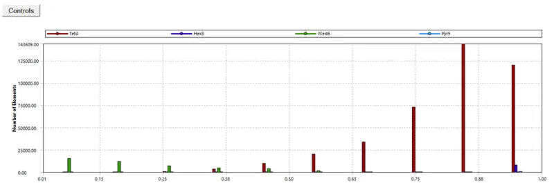
Figure 38: Mesh Quality

Figure 39: Statistics

• Results

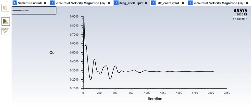
Figure 40: Drag coefficient

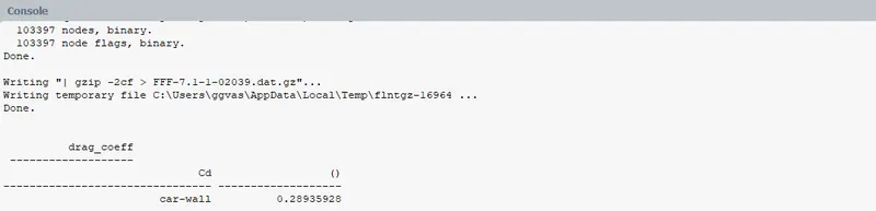
Figure 41: Drag coefficient compute

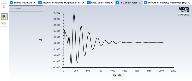
Figure 42: Lift coefficient

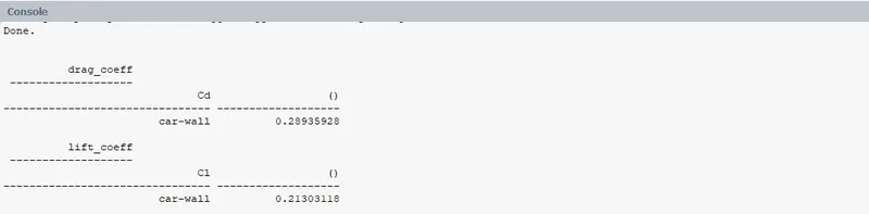
Figure 43: Lift coefficient compute

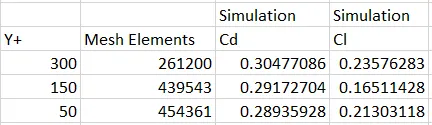
Figure 44: `C_d` and `C_l` at different Y+ values

Post Processing

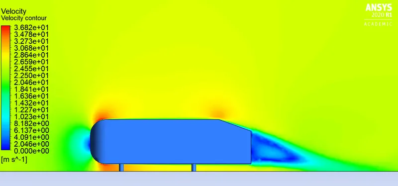
Figure 45: Velocity contours

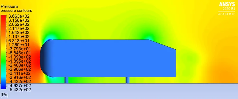
Figure 46: Pressure contours

In the Figure 45 velocity contours are shown. At the nose of the Ahmed body as it is stagnation point, velocity appears to be 0m/s, while at the upper and the lower side of the nose we have approximately the same velocities as the front side of the geometry is symmetrical, Velocities at that region is the highest, causing static pressure to decrease. According to the Bernulli's energy conservation equations, as the pressure consists of two parts: dynamic and static pressure, while dynamic pressure increases, we have a drop in static pressure, The contours in the figure 45 and 46 shows the same, in the regions where the velocity is highest we have the lowest values of static pressure. However, as we look at the rear side of the body we notice that significantly large region has low value of velocity, approximately the same as we had at the stagnation point where the pressure was the highest, but pressure at the rear side of the Ahmed body does not seem no be as high as it is at the stagnation point. At first glance it may be unintuitive, however this fact could be explained by vortex generation phenomenon which forces the airflow vectors to change their direction and start circulation.

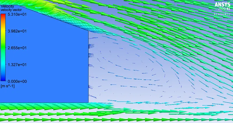
Figure 47: Velocity vectors

In order to clearly show the vortex generation and wake region at the rear side of the Ahmed body, we are using streamlines shown in the Figure 48.

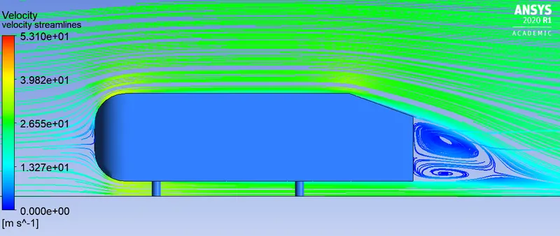
Figure 48: Velocity streamlines

As you see, in the Figure 48 at the back side of the body airflow is recirculated. As the air is penetrated by the Ahmed body at the rear side of the body negative pressure values appear, as the ambient pressure is higher while airflow passes the Ahmed body, due to energy conservation law, which says that every physical propetry tends to flow from a higher value to a lower one, air tries to fill the emptiness at the rear side of the body, that's why flow begins to circulate in that region and is called "Vortex Shedding". The Vortex Shedding is a hugh problem in aerodynamics, therefore there are a lot of concepts to even partially eliminate it. For instance, in "T50" a fan is used at the rear side of the car to blow air flowing at the upperside of the car into the region where the wake is considered to take place, this act decreases pressure difference between the upper and lower ends of the car and the region where the wake is considered to be present.

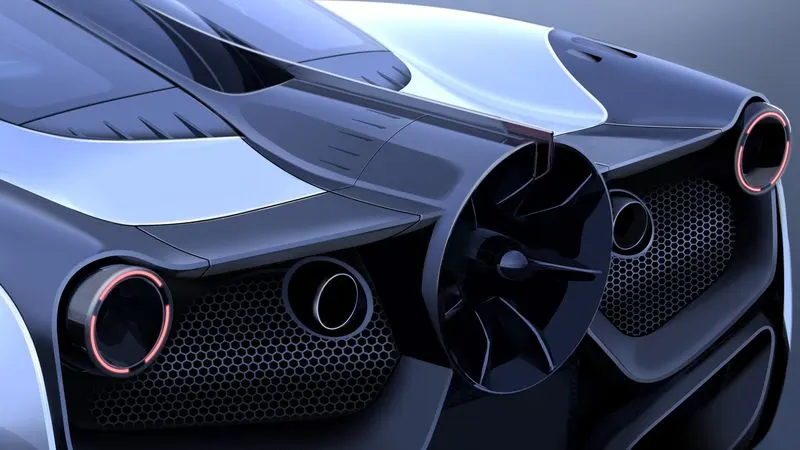
Figure 49: Rear side of a Supercar T50

Other popular option is to change the shape of the rear side of an outomobile. For example, Mclaren Speedtail does it's job perfectly to partially eliminate wake region at the rear side, by making the rear side of the car pointy

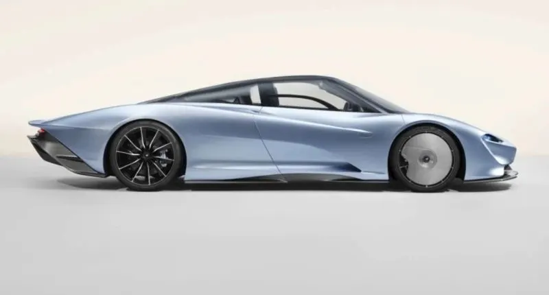
Figure 50: Mclaren Speedtail

This method helps to generate wake region with much less volume.

Conclusion

We successfully simulated mesh independent test of the Ahmed body case. Investigated what causes negative pressure values at the rear side of the body. Furthermore discussed wake region generation and eventually introduced ways how to solve it partially.