Week 9 - Mini project - Flow over an Airfoil

Objective

Simulate flow over a 4 digit airfoil i.e NACA 2412 Airfoil.

• Drag coefficient Vs Angle of Attack
• Lift coefficient vs Angle of Attack
• Compare the effect of turbulence models on the above two results.
• Make sure that the inlet Reynolds number is 200,000
• Make sure you do the above calculations for the following angle of attacks,
  • The angle of attack = 1º
  • The angle of attack = 5º
  • The angle of attack = 10º
  • The angle of attack = 15º

Geometry

To get the .DAT file for the Airfoil, I used the website http://airfoiltools.com/airfoil/naca4digit

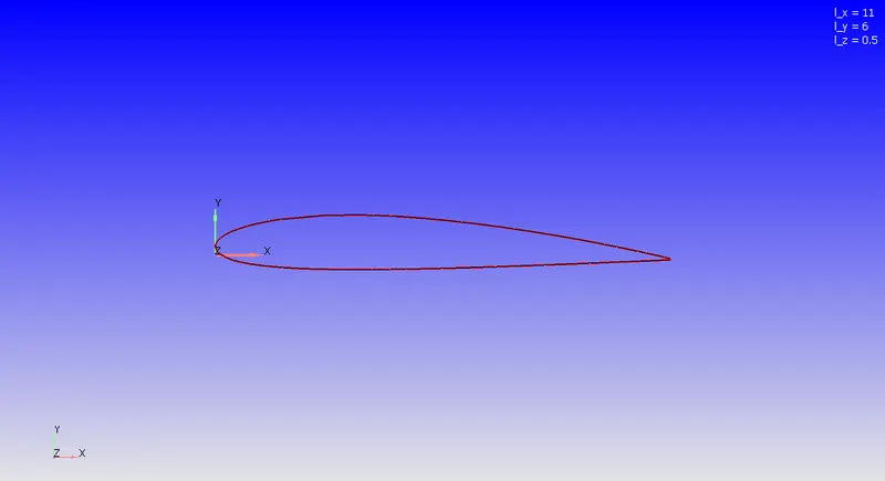
Figure 1

For simulating airfoil aerodynamics It's imperative to create a virtual wind tunnel around the object which is shown in Figure 1. Therefore we created the wind tunnel with specific dimensions with respect to the airfoil itself. The distance in front of the Airfoil is 25 times the cord length of the Airfoil which is 0.2 meters, therefore the distance in front of the Airfoil is 5 meters, moreover, the rear side of the wind tunnel is located at the distance of 30 time the distance of the chord length, therefore 6 meters, furthermore the height of the wind tunnel is 30 times the chord length, thus 6 meters.

• Boundary flagging

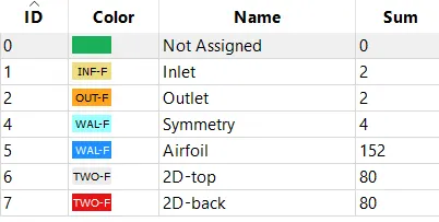
Figure 2

• Inlet

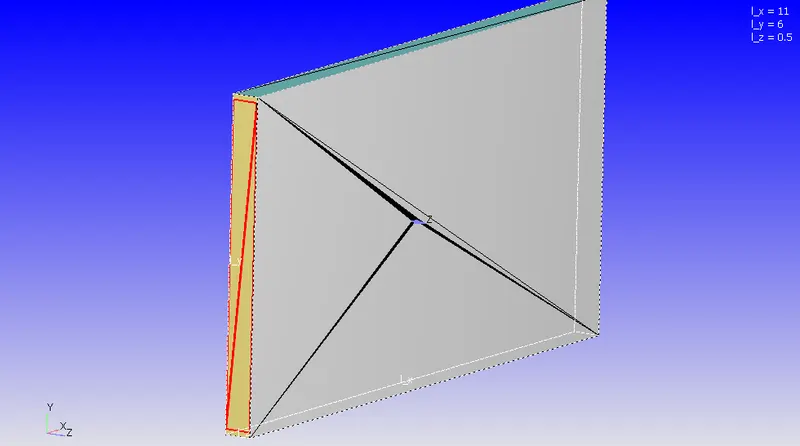
Figure 3

• Outlet

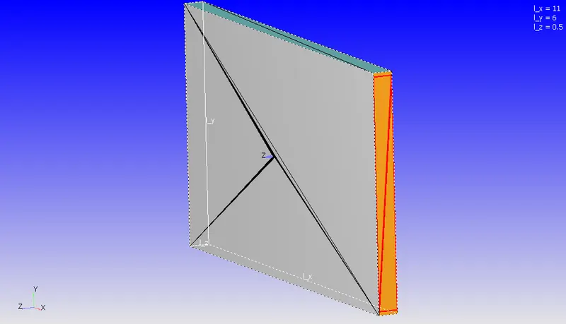
Figure 4

• Symmetry

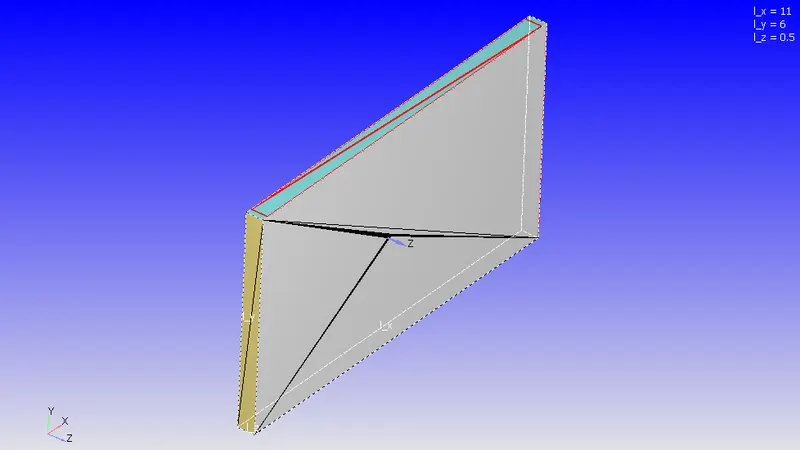
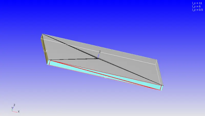
Figure 5

• 2D-top & back

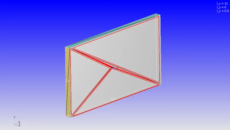
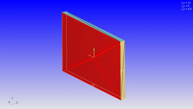
Figure 6

Note: We need 2D-top & back faces in order to simulate a 2-dimensional case.

• Airfoil

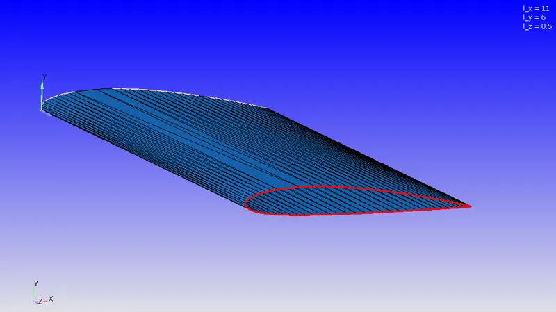
Figure 7

Case setup

• gas simulation (Air). we use real gas as an operating fluid

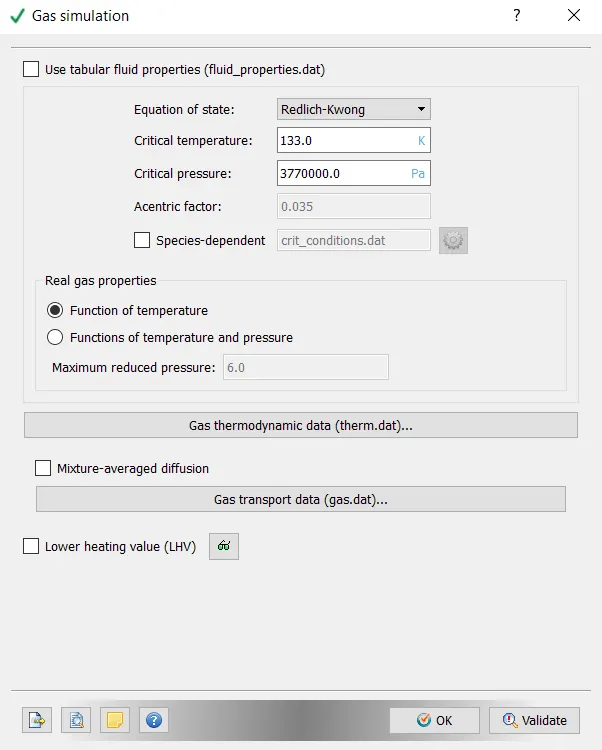
Figure 8

• Run parameters

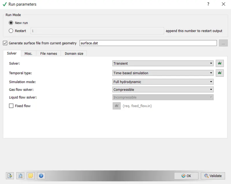
Figure 9

• Simulation time parameters

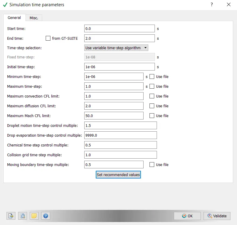
Figure 10

• Boundary conditions

Inlet

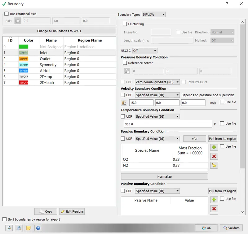
Figure 11

In Figure 11 in Velocity boundary conditions freestream velocity is 15m/s, this value comes from the so-called Reynold's number which should be 200,000 in our case.

1) `Re = 200000 = (rho*v*L)/mu` Where - `rho` is air density

`v` is air velocity

`L` is the characteristic length, chord length in our case.

`mu` is the dynamic viscosity of Air.

2) `v = (Re*mu)/(rho*L) = (200000*0.000017)/(1.225*0.2)=14.6~~ 15`m/s

Outlet

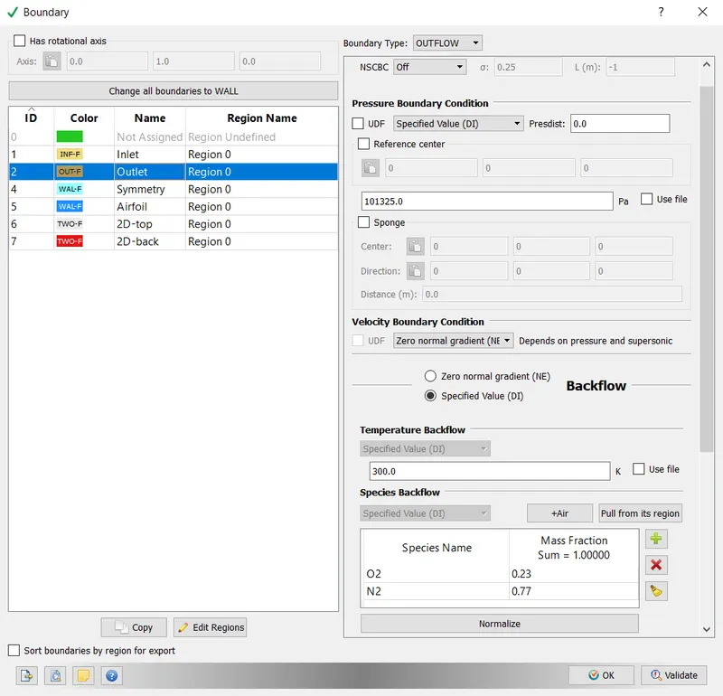
Figure 12

Symmetry

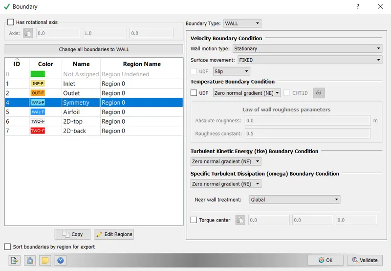
Figure 13

Airfoil

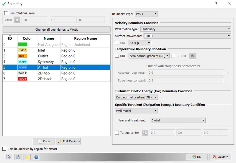
Figure 14

2D

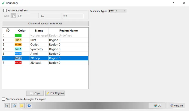
Figure 15

Initialization

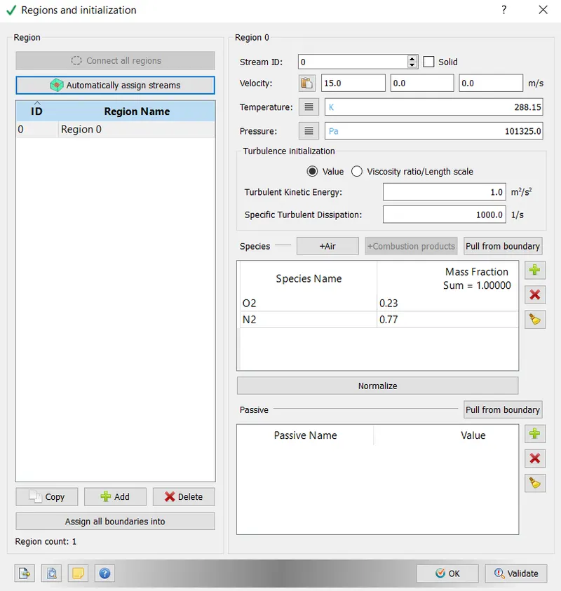
Figure 16

• Turbulence model

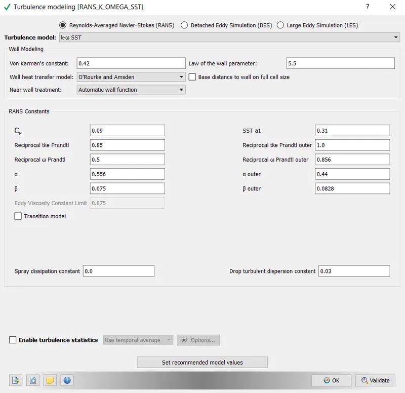
Figure 17

• Meshing

Base grid

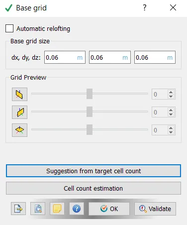
Figure 18

Fixed embedding

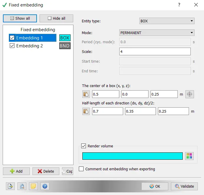
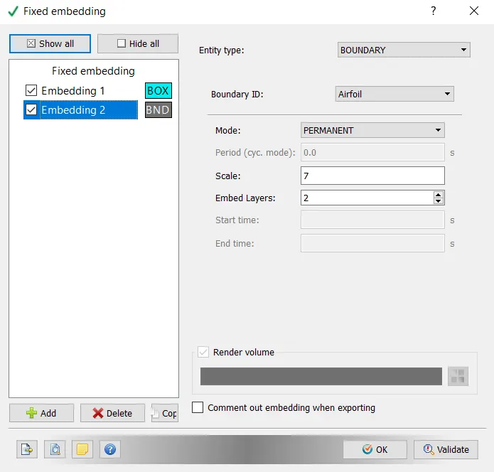
Figure 19

For sufficient analysis, we need fine mesh near the airfoil wall to properly capture the turbulent boundary layer generation and predict drag and lift forces.

Nondimensional distance Y+ is an important parameter to capture near-wall fluid flow. While Y+ is in the range of 0 to 1 we call it viscous sub-layer, from 1 to 10 it's buffer layer and from 10 It's called Log-law region in other words, the law of the wall. We need our Y+ value to be 30.

Using the website https://www.pointwise.com/yplus/index.html we can calculate the first layer size for desired Y+ value.

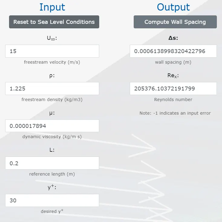
Figure 20

According to figure 20, the first layer size should be 0.0006m. Therefore we use a fixed embedding feature at the airfoil wall. As shown in Figure 19 at the airfoil wall we have a scale of 7, which means that the base grid size will be dived to `2^n`, therefore the first layer size will be `0.06/2^7 = 0.00046875`which is less than the required value for the Y+ of 30.

• Mesh

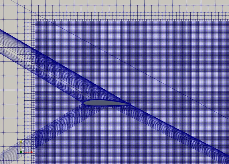
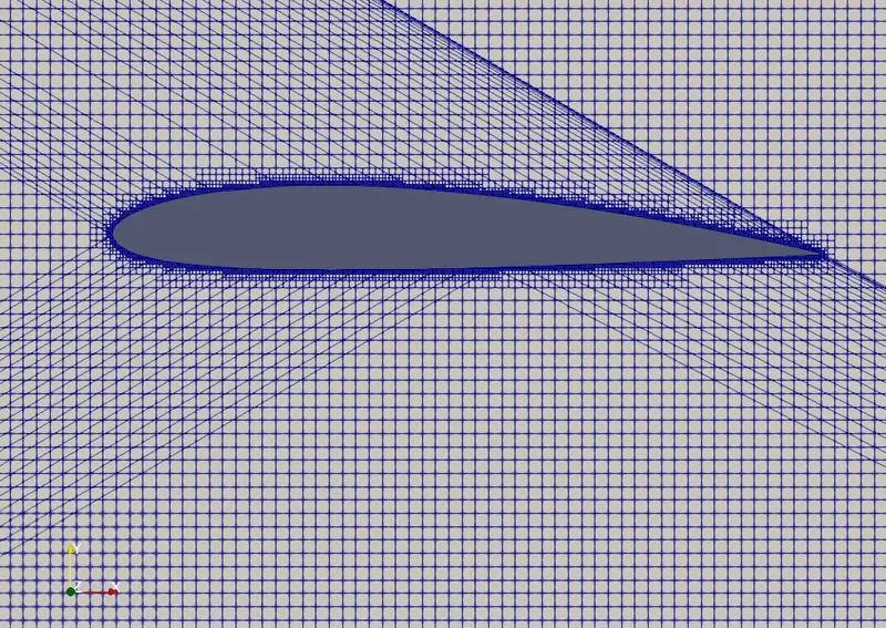
Figure 21

Post-processing

Lift force for all angles of attack

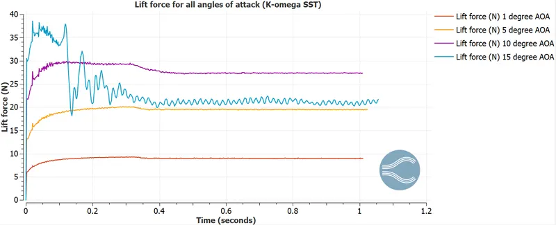
Figure 22

In Figure 22 lift force for all 4 angles of attack is shown, as you see while angle of attack increases from 1 to 10 degrees lift force increases, however at a 15-degree angle of attack the Airfoil stalls and the lift force drops significantly.

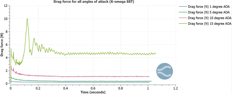
Figure 23

Figure 23 shows that while increasing the angle of attack Drag force increases, moreover while the airfoil stalls at the 15-degree angle of attack we see a huge jump in the Drag force from a 10 to 15-degree angle of attack.

In order to plot lift & drag coefficients and angle of attack dependence, initially, we should calculate lift & drag coefficients.

3) `C_f = (2L)/(rho*v^2*S)` Where - `C_f` is lift force coefficient

`L` is lift force

`rho` is density

`v` is velocity

`S` is airfoil surface area

4) `C_d = (2D)/(rho*v^2*S)` Where - `C_d` is drag force coefficient

`D` is drag force

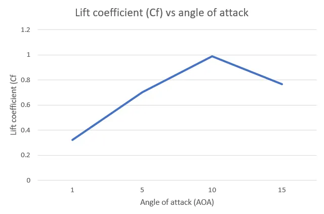
Figure 24

In Figure 24 lift coefficient and angle of attack, dependence is shown, according to the plot we find out that at the 15-degree angle of attack airfoil stalls and we experience a significant drop in lift force.

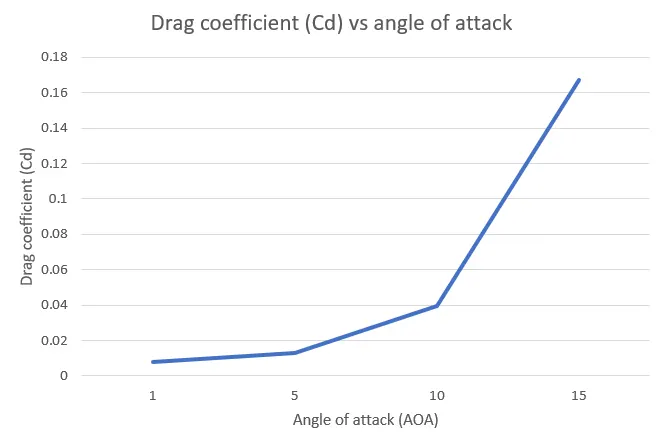
Figure 25

turbulence models (RNG K-`epsilon` & K-`omega` SST)

RNG K-`epsilon` model two-transport equation solving for turbulent kinetic energy K and turbulent dissipation `epsilon`. This model is valid for only fully turbulent flows and is applicable for freestream flows, whereas K-`omega` SST (shear stress transport) model is a two-transport equation model solving for kinetic energy K and turbulent frequency `omega`. This model allows for more accurate near-wall treatment. Combines the original Wilcox k-w model for use near walls and the standard k–ε model away from walls using a blending function. That's why in our case we used K-`omega` SST model, however for demonstration we simulated the case using RNG K-`epsilon`.

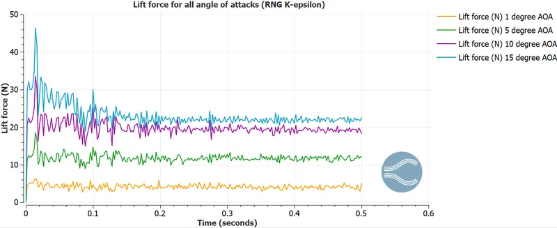
Figure 26

As shown in Figure 26 as the angle of attack increases Lift force increases as well, even at a 15-degree angle of attack airfoil does not experience stall which is considered to be incorrect. That's why we use K-`omega` SST model for analysis.

Conclusion

we successfully simulated the airfoil problem. performed 4 cases at a different angle of attacks, detected the point when the wing stalled. discussed 2 turbulent models and realized benefits of the K-`omega` SST model in our case.