Mixing efficiency

Objective

To simulate and understand working principle of a mixing tree. Run grid dependence test to choose the mesh grid size for further study. In the provided report we will cover 2 cases:

Case1: Short mixing tree with a hot inlet velocity of 3m/s. Momentum ratio between hot and cold inlets are 2 and 4, meaning cold inlet velocity divided by hot inlet velocity equals to the Momentum ratio.

Case2: Long mixing tree with a hot inlet velocity of 3m/s. Momentum ratio between hot and cold inlets are 2 and 4, meaning cold inlet velocity divided by hot inlet velocity equals to the Momentum ratio.

Case 1 setup (short pipe)

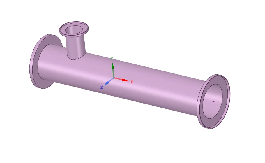
• Geometry (Solid zone)

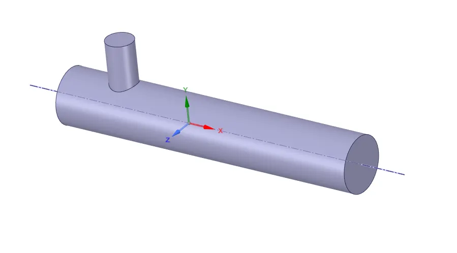
• Geometry (Fluid zone)

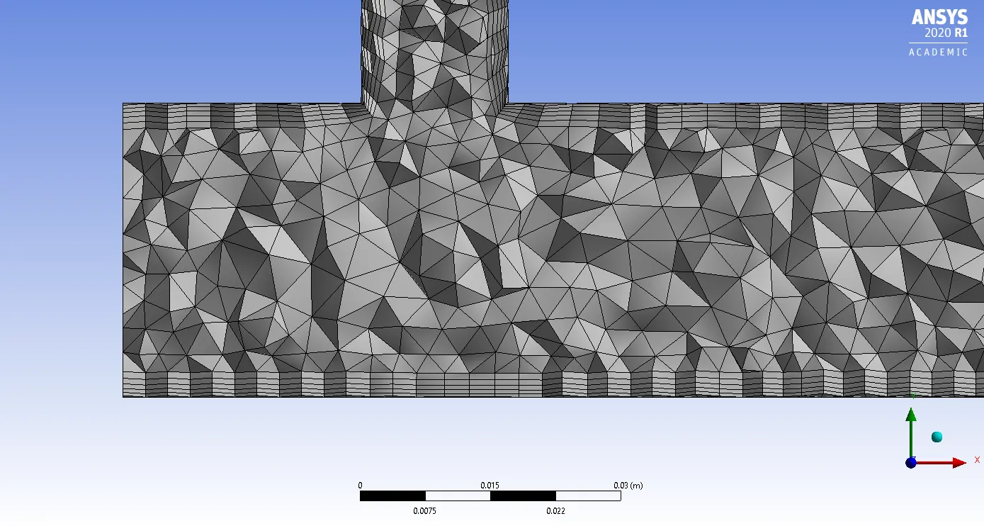
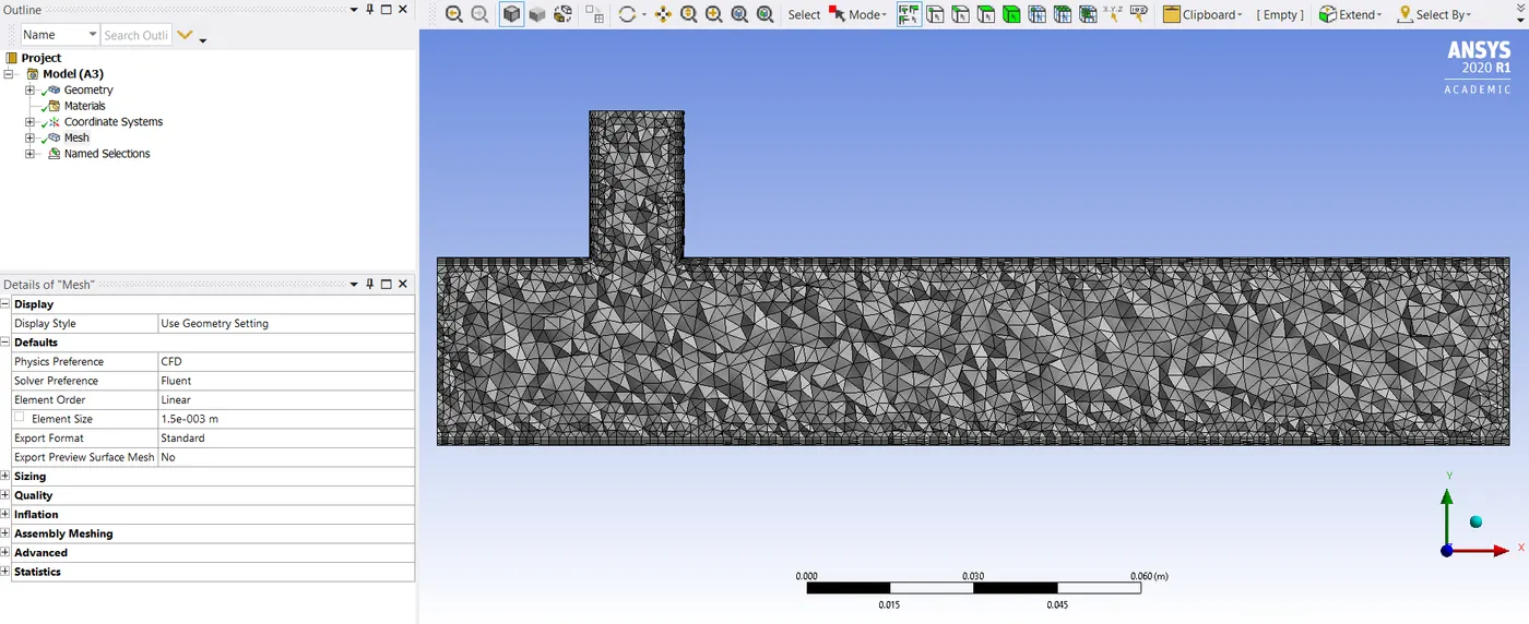
• Mesh

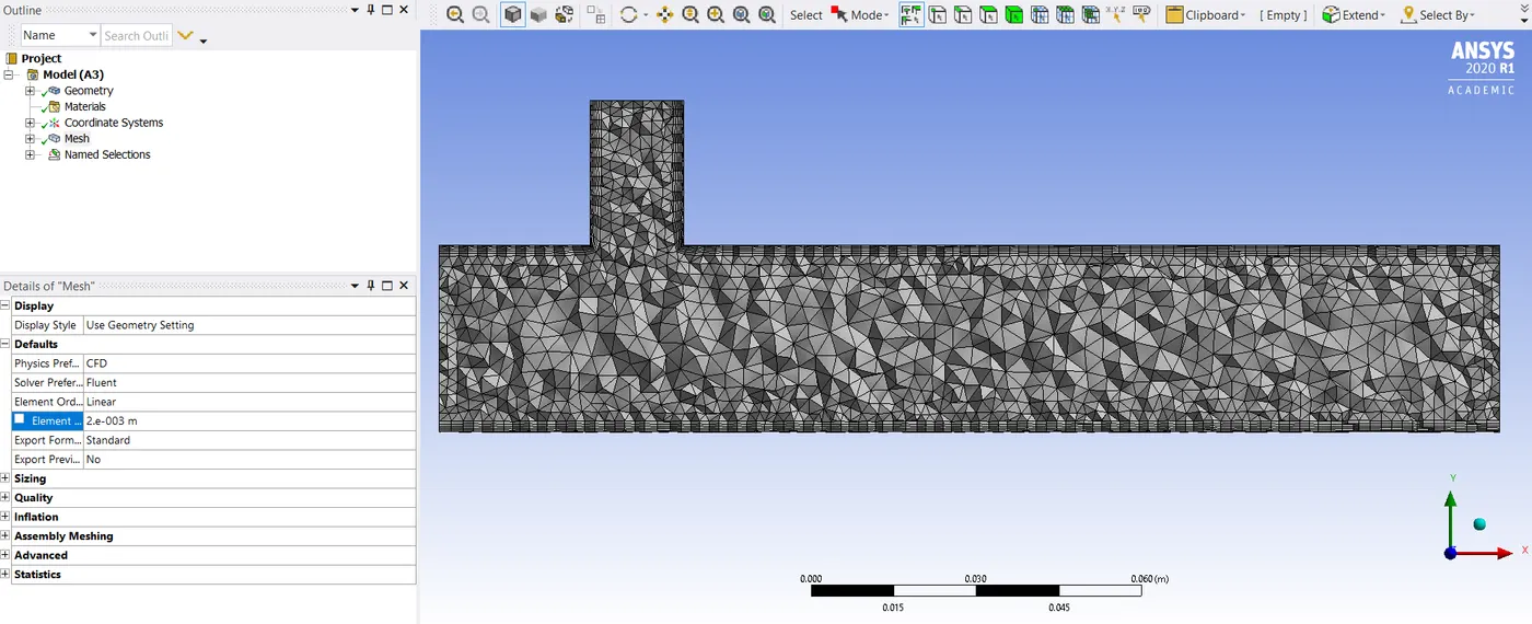
While generating mesh as an element size initially we choose 3mm.

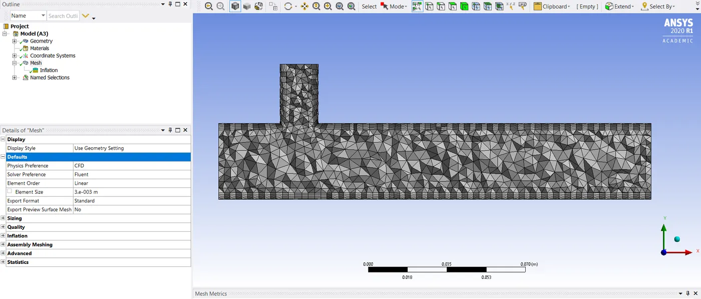
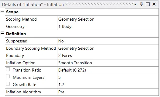
In addition we include inflation layers near the walls as well.

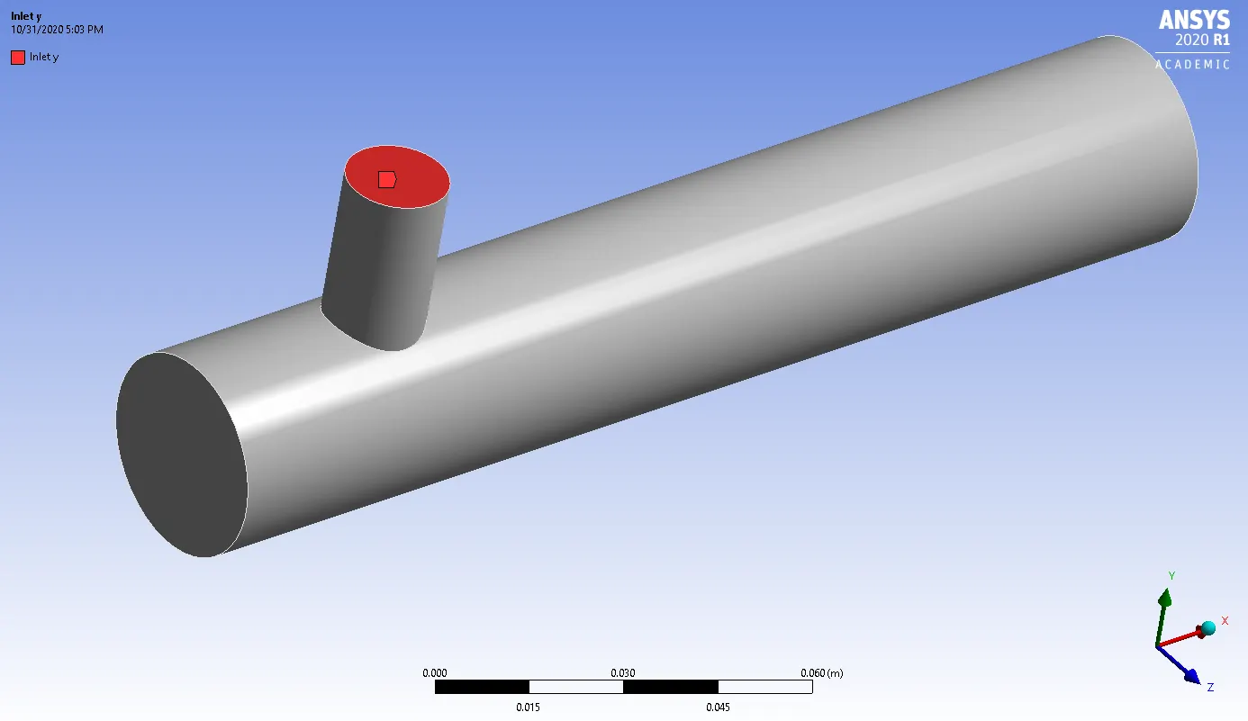
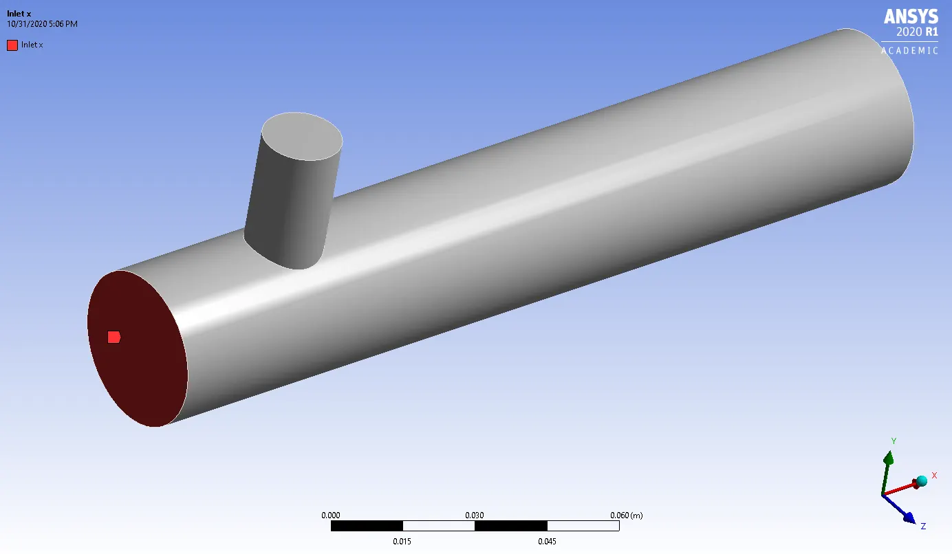
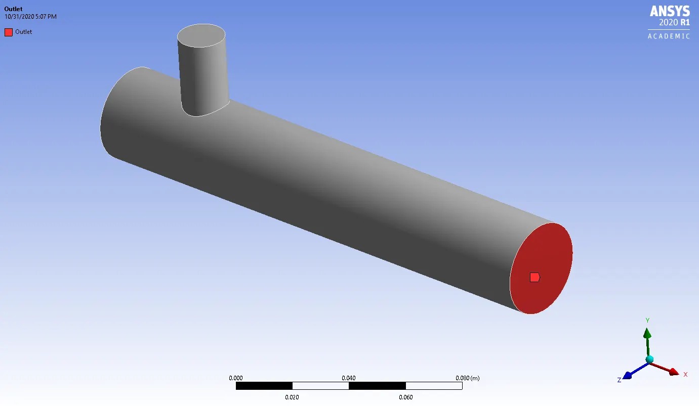
• Named selections

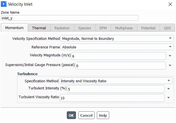
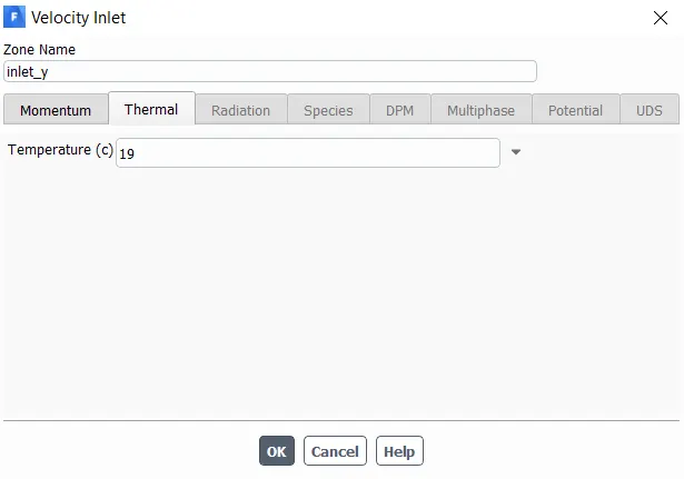
Inlet y (cold air inlet)

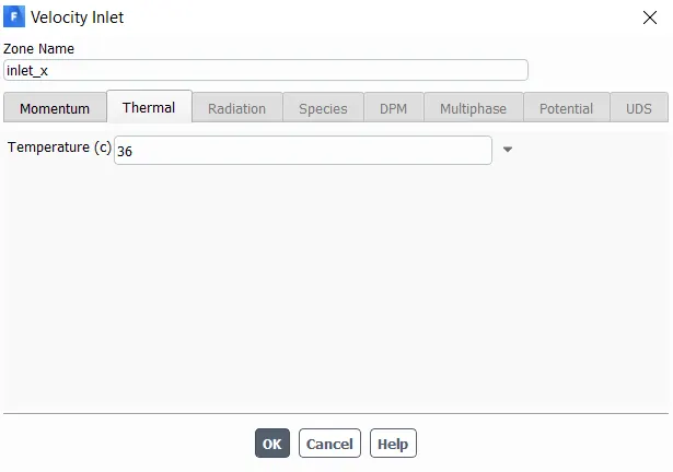
Inlet x (Hot air inlet)

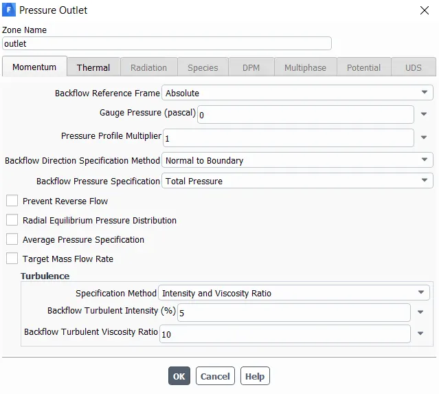
Outlet

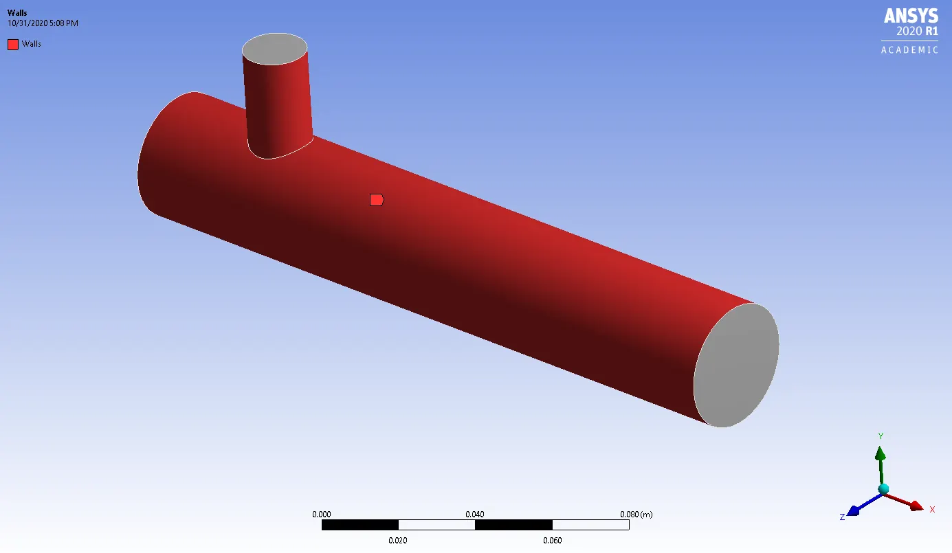
Walls

• ANSYS Fluent physics set up and solution.

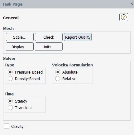
In our case due to low values of velocity we can have a pressure-based type of the solver. We are solving with steady state solver to see the mean value of temperature at the outlet when the simulation reaches steady state.

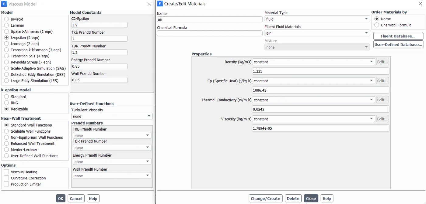
As a turbulent model we are using Realizable K-epsilon solver with the standard wall functions. As a fluid, we have ideal gas (air).

• Initial and Boundary Conditions.

Inlet x

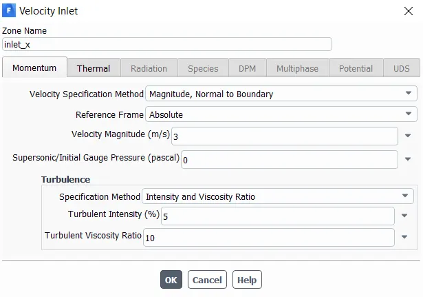
Inlet y

Outlet

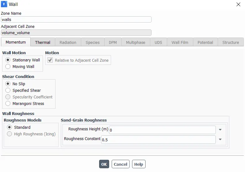
Walls

• Report definitions

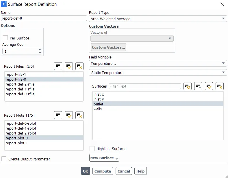
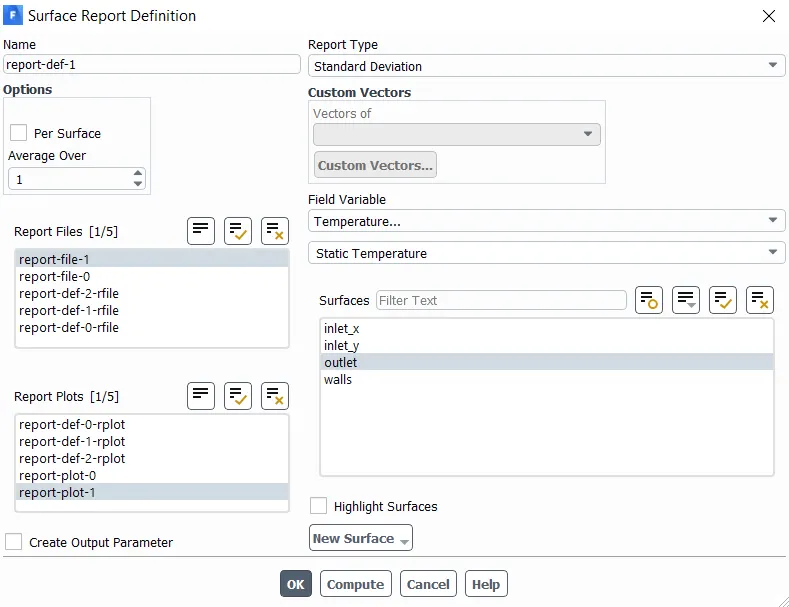
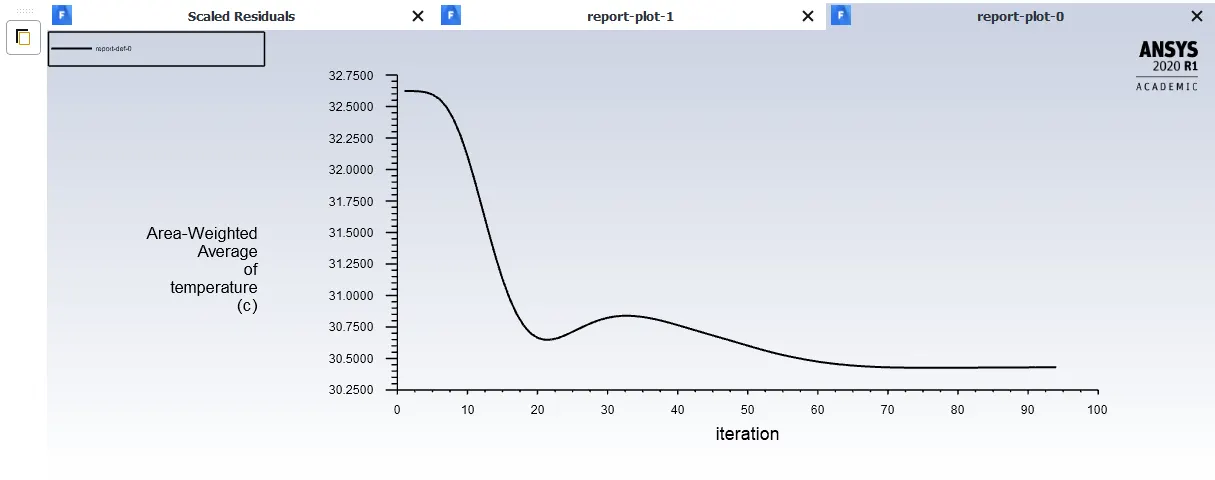
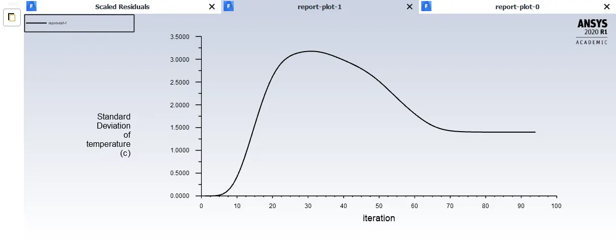
We are monitoring 2 different values at the Outlet: The first value is the Area-weighted Average of the temperature and the second one is the standard deviation of the temperature at the outlet.

• Computational residual values

• Result plots

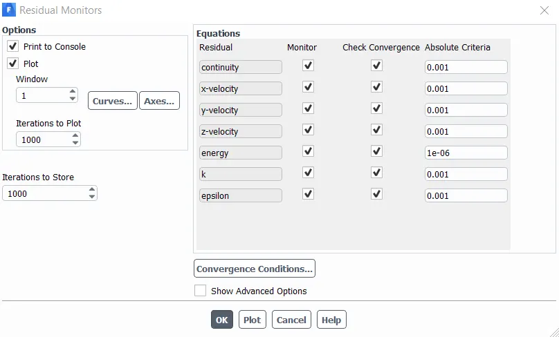
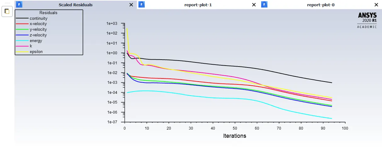
Scaled residuals

Area-weighted Average

Standard deviation

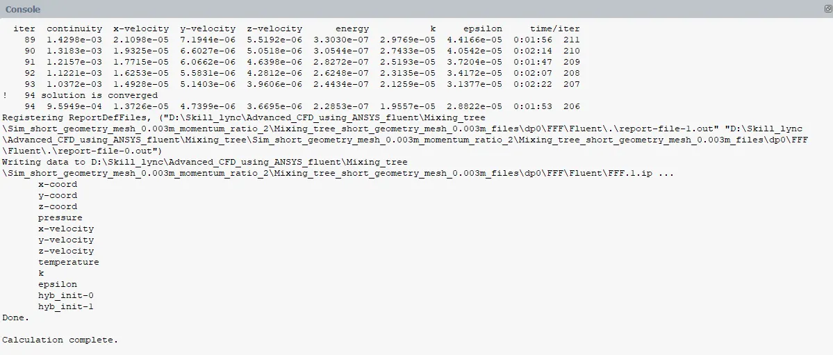
Number of iterations

• Post processing

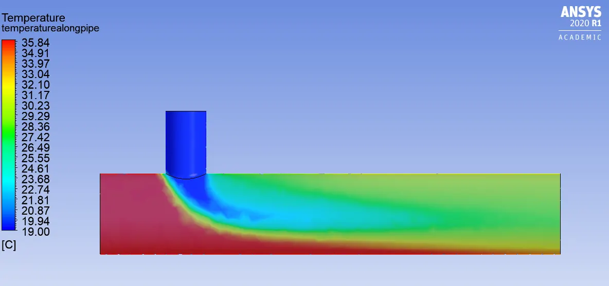
Temperature contours

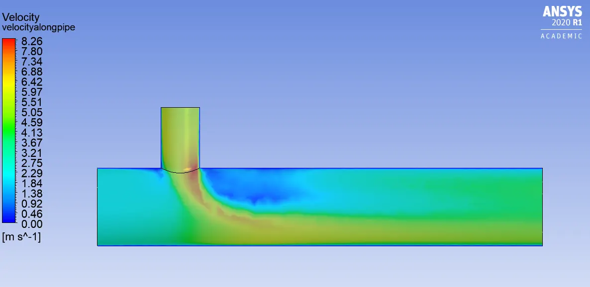
Velocity contours

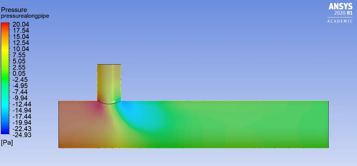
Pressure contours

After completing the first case we run mesh dependence test. As you know initially mesh size was 3mm, afterwards we generated mesh with different values of element sizes: 2mm and 1.5mm and run the simulation for each of the mesh size.

• 2mm case

• Result plots

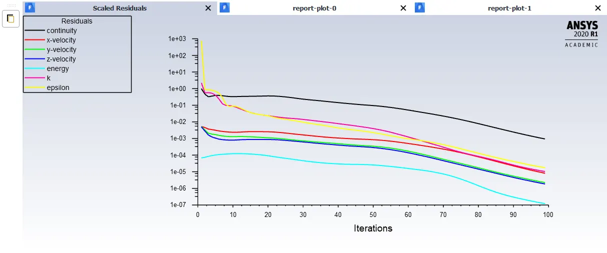
Scaled residuals

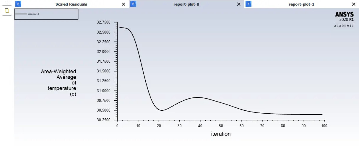
Area-weighted Average

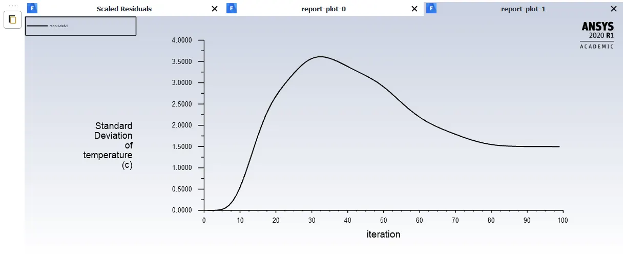
Standard deviation

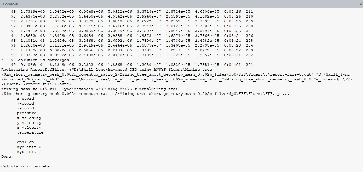
Number of iterations

• Post processing

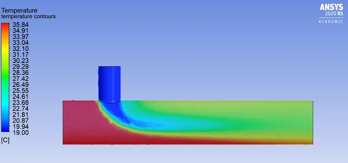
Temperature contours

• 1.5mm case

• Residual plots

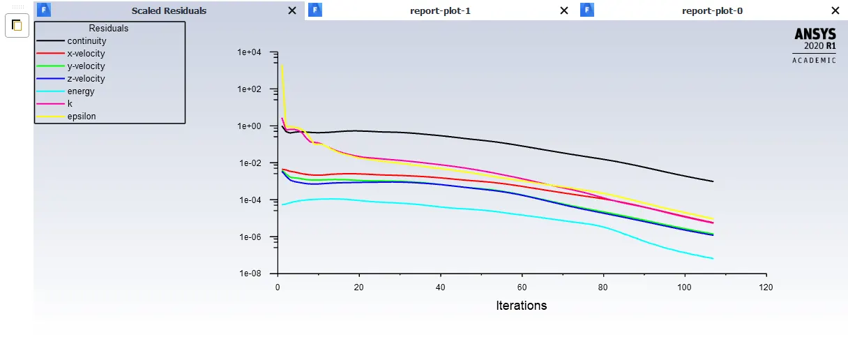
Scaled residuals

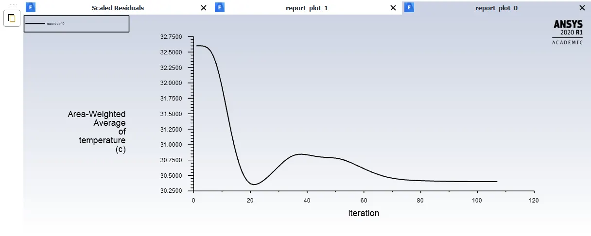
Area-weighted Average

Standard deviation

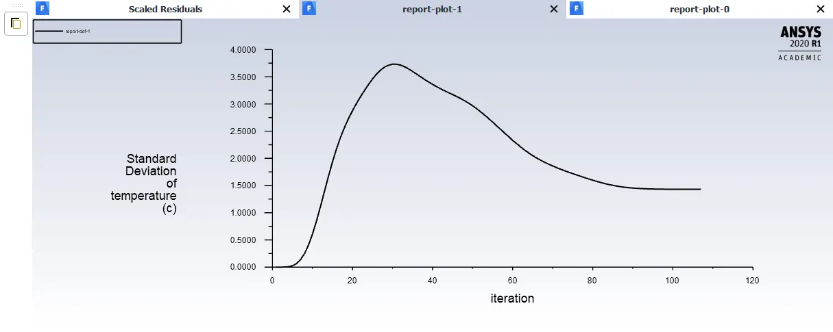
Number of iterations

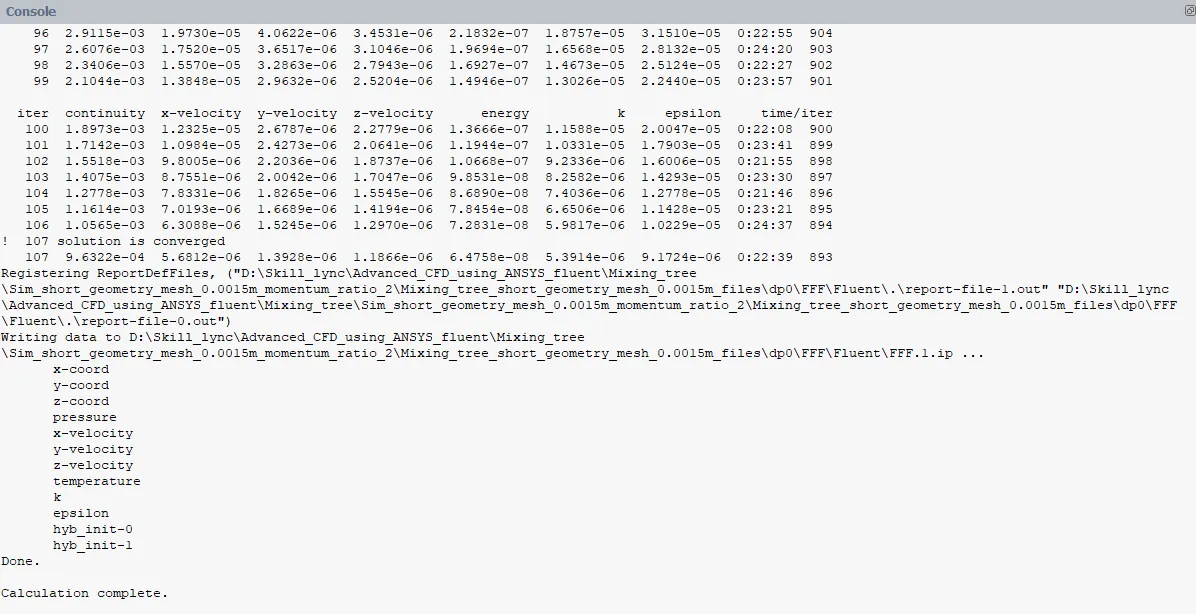
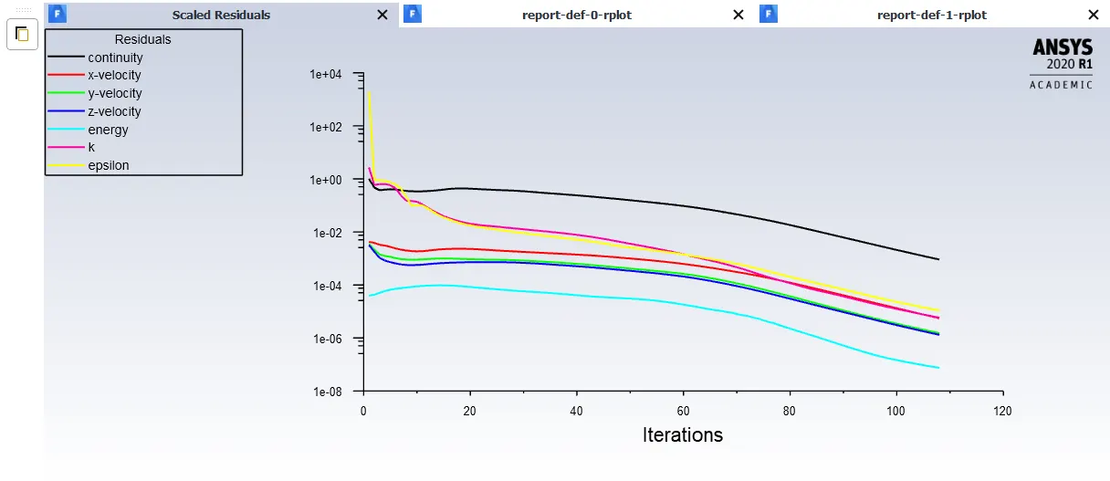
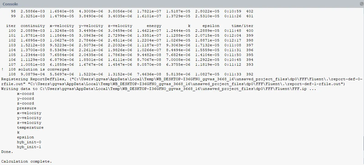
According to the Result plots for all 3 meshes we found out that Area-weighted average and standard deviation of temperature is approximately the same, therefore we can conclude that we can use mesh size to be 3mm, however due to problem low complexity time consumed for solving the simulation is negligible, thus we are using 1.5mm mesh in order to provide smooth contours while showing the results. In addition, we should include that while increasing the number of the mesh elements solver converges in more iterations, which is intuitive. For the 3mm mesh case the simulation converged after 94 iterations, As for 2mm case it took 99 iterations to converge and finally for 1.5mm case iteration number was 107.

• Momentum ratio of 2 case

Hot inlet velocity is 3m/s while cold inlet velocity appears to be 6m/s

Temperature contours

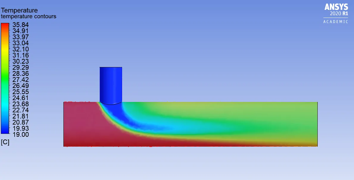
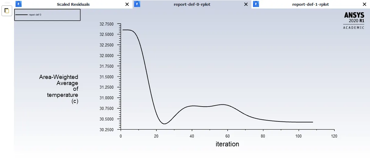
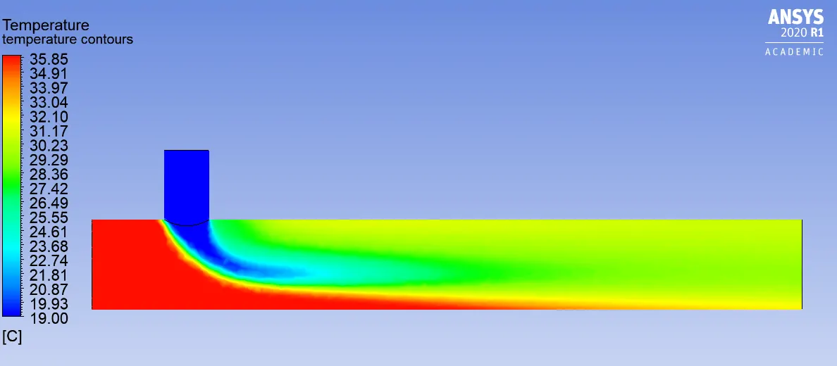
From the figure above it's clear that after mixing cold and hot air we have a mean value of the temperature which is approximately 30.4C.

Temperature contours at the outlet

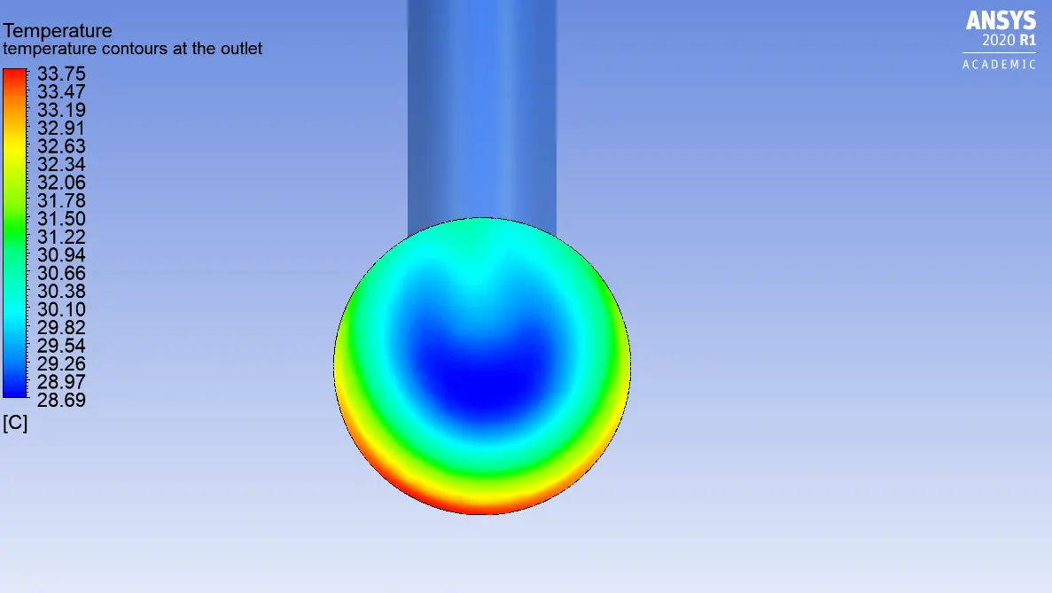
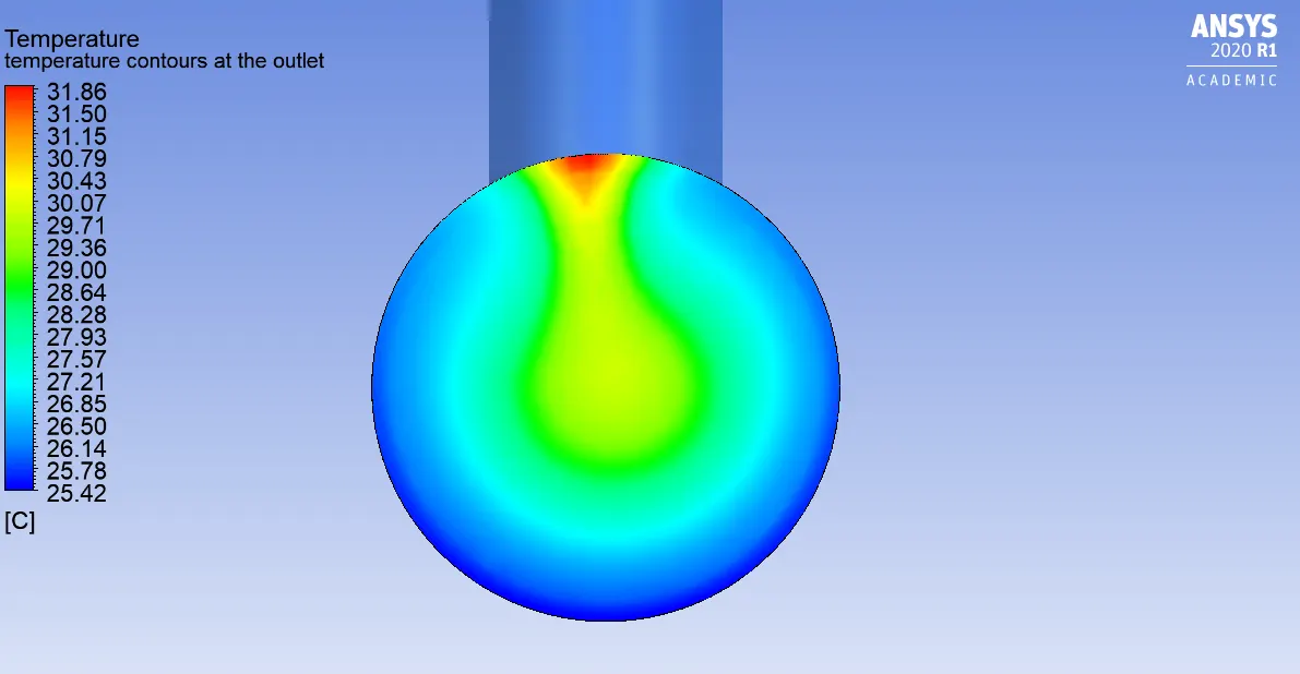
In the mixing tree our goal is to get as uniform temperature profile at the outlet as possible. From the figure above it's clear that temperature profile is not uniform, subsequently we will test the cases with the momentum ratio of 4 and with the longer pipe to figure out if any above mentioned ways really matters.

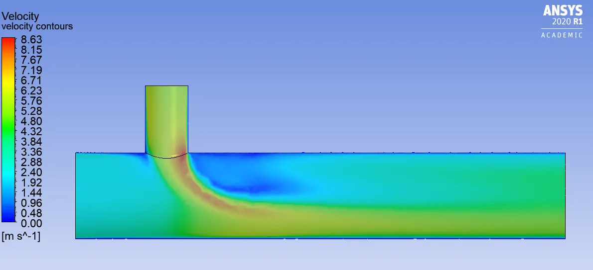
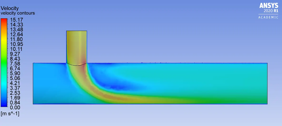
Velocity contours

Pressure contours

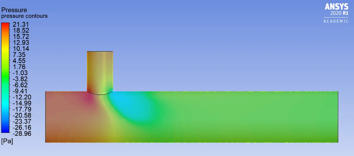
As we see from the pressure contours figure, we can conclude that as the cold air enters and mixes with the hot air due to temperature difference, therefore pressure difference vortex is generated (right side of the cold inlet section)

In that area where we encounter lowest value of pressure, according to the energy conservation velocity must be highest, however from the velocity contours figure we see that in that region velocity is lowest as well. All this is coused due to vortex generation which leads flow to both pressure and velocity decrease (air diffusion is lowest in that region).

• Momentum ratio of 4 case

Hot inlet velocity is 3m/s while cold inlet velocity appears to be 12m/s

• residual plots

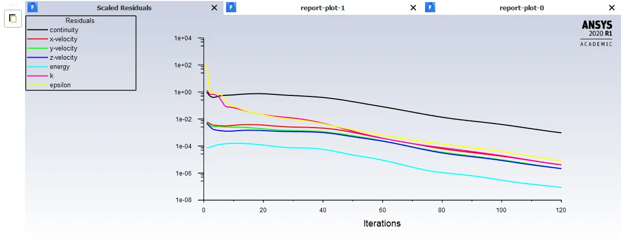
Scaled residuals

Area-weighted Average

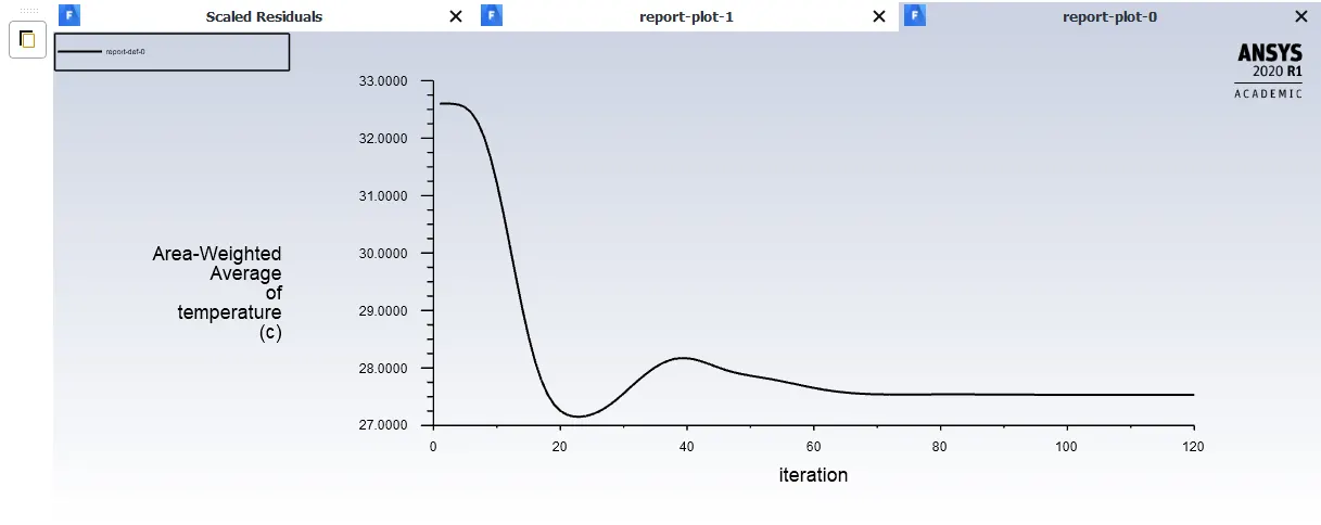
It's clear that as we increased the velocity of the cold air mass flow also increased caused the mean value of the temperature at the outlet to decrease.

Standard deviation

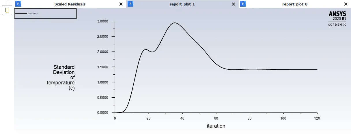
Standard deviation tends to be almost the same as it used to be in the momentum ratio of 2 case.

Number of iterations

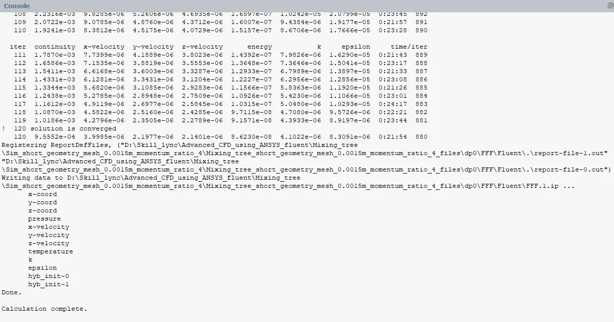
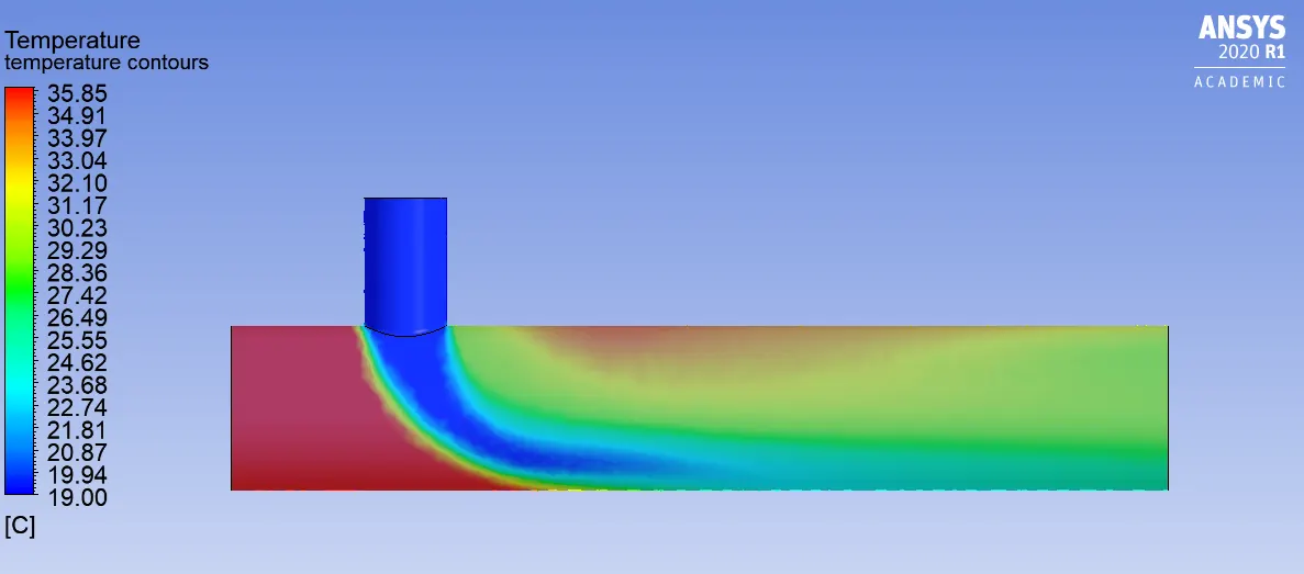
Temperature contours

Temperature contours at the outlet

Velocity contours

Case 2 setup (long pipe)

In this case everything is the same, however we are using a different geometry (Longer pipe).

• momentum ratio of 2 case.

• residual plots

Scaled residuals

Number of iterations

Area-weighted Average

Standard deviation

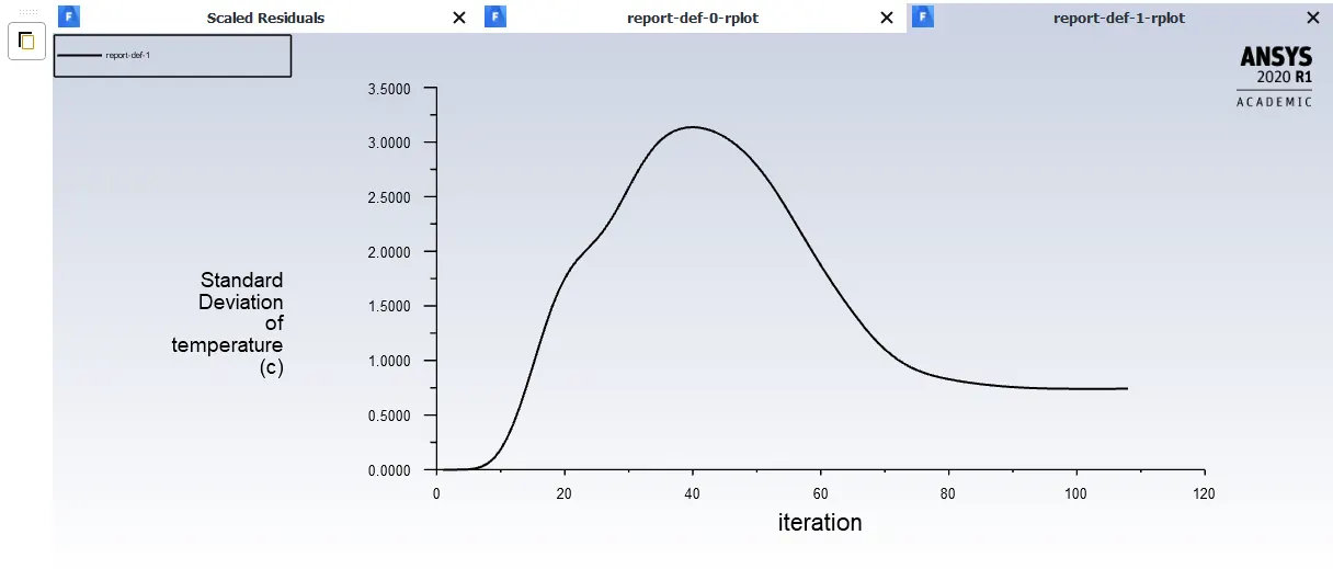
It'sa clear that the pipe length only affect standard deviation of temperature at the outlet. Fortunately it decreases from approximately 1.5 to less than 1 celsius. As for the mean value of the temperature did not change.

Temperature plots

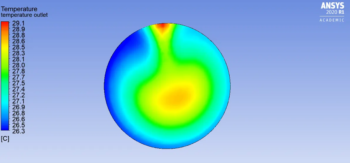
Temperature contours at the outlet

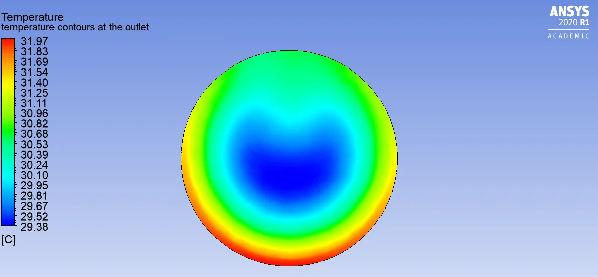
In this case it's noticable that the temperature profile at the outlet is more uniform.

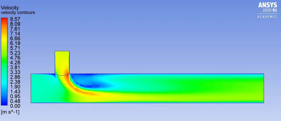
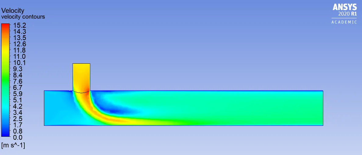
Velocity contours

• momentum ratio of 4 case.

• residual plots

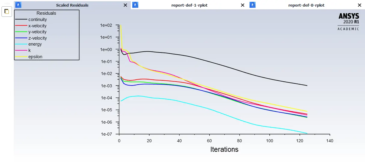
Scaled residuals

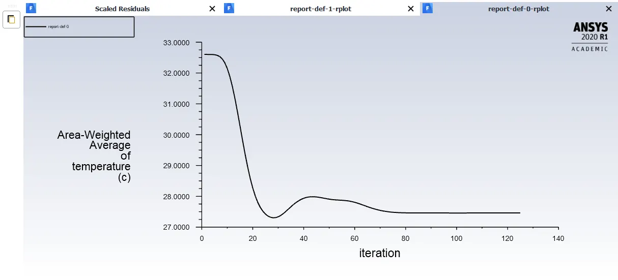
Area-weighted Average

Standard deviation

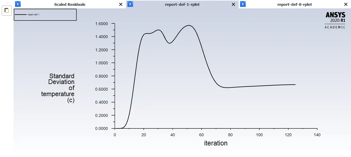
We can say the same for this case as well. Area-weighted Average remains to be the same compared with the same case just with the short pipe, however standard deviation went from 1.5 to 0.7 celsius.

Temperature contours

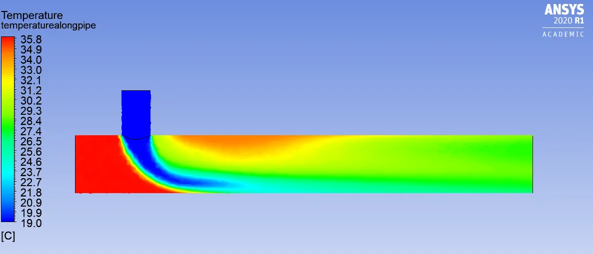
Temperature contours at the outlet

Velocity contours

Conclusion

As we simulated all the cases, realized that cold inlet velocity affects the mean value of the temperature at the outlet, moreover the length of the pipe ensures the uniformity of the temperature profile at the outlet.