Week - 10 Hyperelastic Material Models

λ1=1+ε

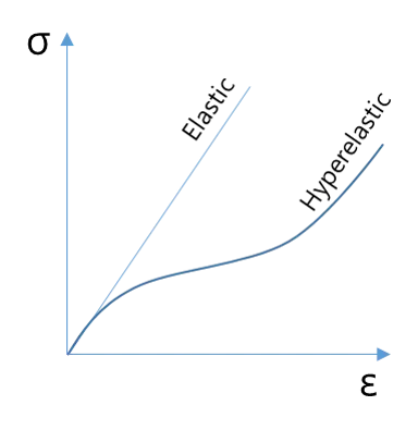
An elastic material is a linear material. This means that stress varies linearly with respect to strain. This material model is accurate for many material models, such as paper, metal, and wood, as long as the deformation is very small.

STRETCH RATIO The stretch ratio or extension ratio is a measure of the extensional or normal strain of a differential line element, which can be defined at either the undeformed configuration or the deformed configuration. It is defined as the ratio between the final length ℓ and the initial length L of the material line

Hyperelastic materials are designed for modeling rubber or rubber-like materials in which the elastic deformation can be extremely large.

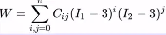
Strain energy density functions (W) establish the relationship between the amount of energy employed to deform a volume unit of a solid and imposed strain.

Usually, stress-strain curve data from experimental tests are used to fit the constants of theoretical models, thus approximating the material response.

The choices of hyperelasticity models :

1. Neo-Hookean (first-order reduced polynomial)
2. Mooney-Rivlin (first-order complete polynomial)
3. Odgen(second-order reduced polynomial)

NEO-HOOKEAN:-

Odgen:-

https://www.simscale.com/docs/simulation-setup/materials/hyperelastic-materials/

Procedure:

• In this model, they had given the engineering stress vs engineering strain file.
• We need to convert the image stress and strain values into an xl file.

ENG STRAIN	ENG STRESS
0.00E+00	0.00E+00
2.50E-02	4.46E-02
5.00E-02	8.67E-02
7.50E-02	1.27E-01
1.00E-01	1.64E-01
1.25E-01	2.00E-01
1.50E-01	2.34E-01
1.75E-01	2.67E-01
2.00E-01	2.98E-01
2.25E-01	3.28E-01
2.50E-01	3.56E-01
2.75E-01	3.83E-01
3.00E-01	4.09E-01
3.25E-01	4.34E-01
3.50E-01	4.58E-01
3.75E-01	4.81E-01
4.00E-01	5.03E-01
4.25E-01	5.24E-01
4.50E-01	5.45E-01
4.75E-01	5.65E-01
5.00E-01	5.84E-01
5.25E-01	6.03E-01
5.50E-01	6.20E-01
5.75E-01	6.38E-01
6.00E-01	6.55E-01
6.25E-01	6.71E-01
6.50E-01	6.87E-01
6.75E-01	7.02E-01
7.00E-01	7.17E-01
7.25E-01	7.32E-01
7.50E-01	7.46E-01
7.75E-01	7.60E-01
8.00E-01	7.73E-01
8.25E-01	7.86E-01
8.50E-01	7.99E-01
8.75E-01	8.11E-01
9.00E-01	8.23E-01
9.25E-01	8.35E-01
9.50E-01	8.47E-01
9.75E-01	8.58E-01
1.00E+00	8.69E-01

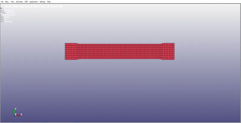
• After the calculations, we need to open the ls pre-post with the given model.

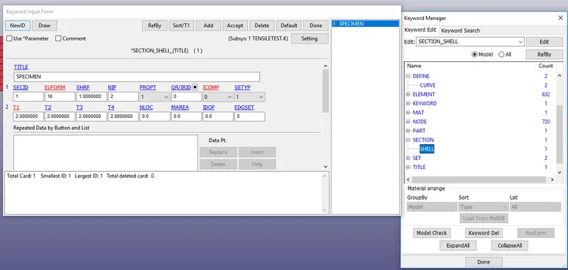
• We need to create a section for the part to define element formulation.
• Here we selected the section as 16 as fully integrated and thickness as 2mm.

• After creating the material and section we need to combine to part.
• Then we need boundary conditions like fixing the one end and another end we need to give the curve of displacement.
• To make constrained select to create an entity and select boundary conditions and select SPC and lock all directions, except in y to get compressible behavior.

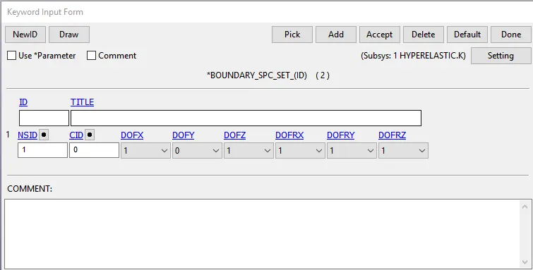
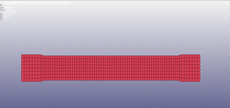
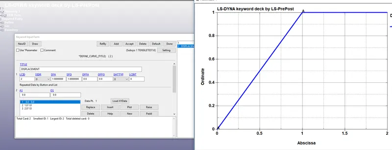
• From prescribed motion, we need to provide displacement vs time graph.
• To define go to define and input the x,y values and save them.
• Here we need o give the scale factor Sfo as 145.

λ=1+ε (strain=100%,ε=1)

λ=2, L=145

ε=∂l/l

∂L=145mm

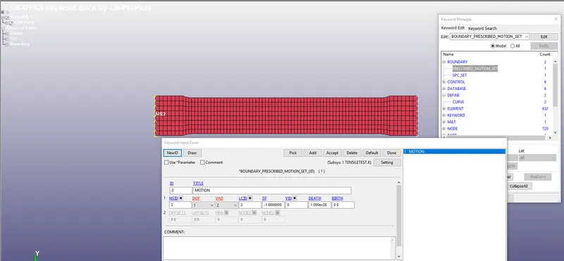
• Go to prescribed motion set and make node as a set and import the curve and give VAD=2 and save it.

• For this simulation, we are going to use only the implicit solver.
• To activate the implicit solver we need to select control implicitly and select IMFLAG as 1.
• The solver will be activated and we can give the initial time step to start.
• Here we had given the initial time step as 0.01ms.

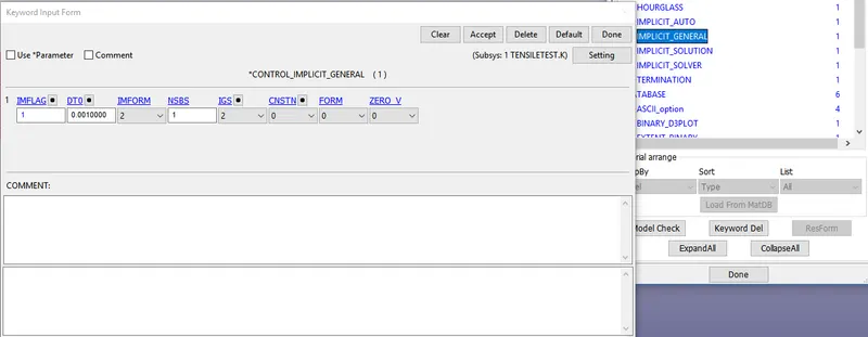
• And we need to activate the auto time step to increase the chance of convergence.
• And also we can constrain the number of iteration to be solved.

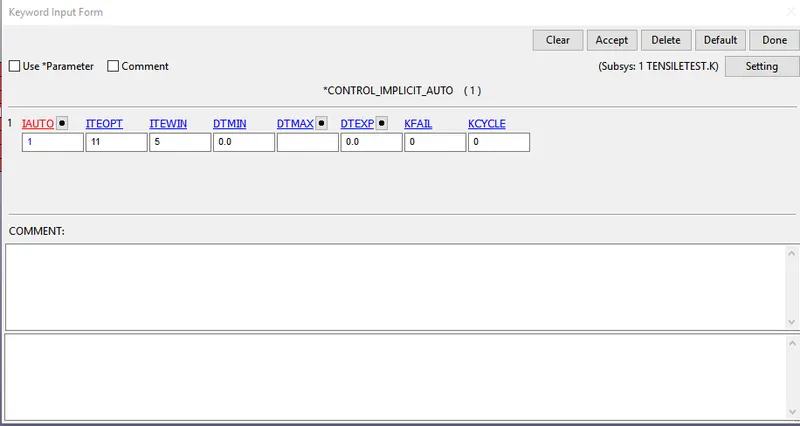
ITEOPT: Optimum equilibrium iteration count per time step.

ITEWIN: Allowable iteration window. If iteration count is within ITEWIN

iterations of ITEOPT, the step size will not be adjusted for the next

step.

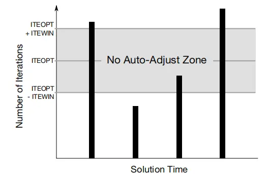
• For a certain time step if the solver is converging in less number of the steps then the time step will automatically increase.
• If it is unable to solve for that time step it will increase the iterations.

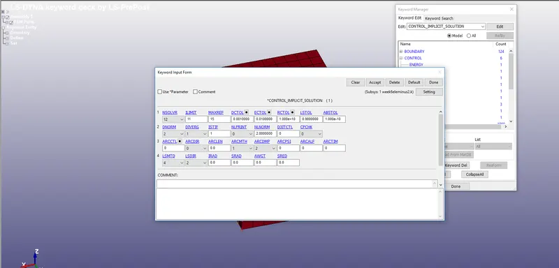
• CONTROL_IMPLICIT_SOLUTION:-These optional cards apply to implicit calculations. Use these cards to specify whether a linear or nonlinear solution is desired.

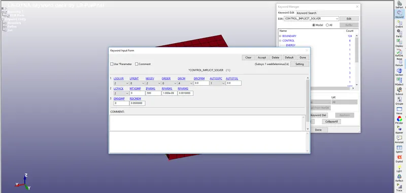
• CONTROL_IMPLICIT_SOLVER:-These optional cards apply to implicit calculations. The linear equation solver performs the CPU-intensive stiffness matrix solution.
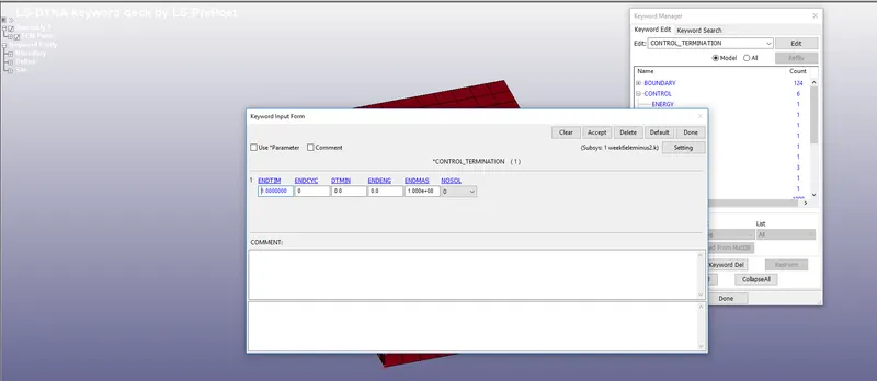
• We need to give the end termination time to solve.

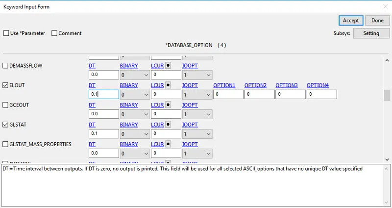
• We need to give output requests to get results from the post-processor.

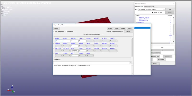
• This is used to get the strain result from the elements STRFLG=1.
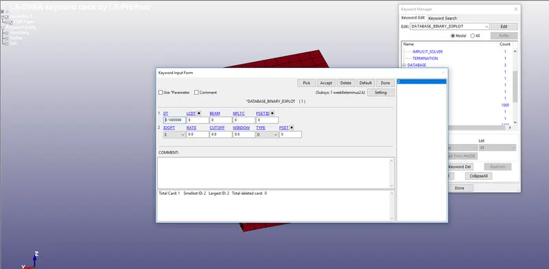
• And we need to give access to binary d3plot and In ASCII glstat.

To give an output request we need to go to the database and give ASCII and BINARY POLT.

• ELOUT:-database for element results for SSD (stress and strain
  components).
• D3PLOT:-Database for the entire model.
• GLSTAT:- file is the sum of internal energy of discrete elements.
• MATSUM:- Energy values part by part.
• SPCFRC:-Single point force constrained
• SWFORC:- Spot weld forces

• Then we need to go to keyword and select MAT 77(Hyperelastic material)
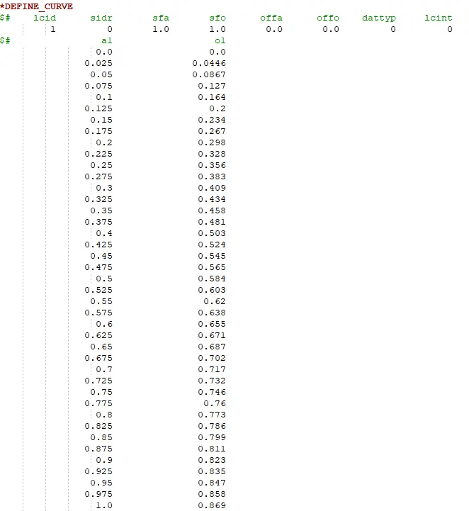
• To give that we need to define the curve.
• Here we can define the curve from the .k file by pasting the value at curve positon
• By using alt we need to arrange value systematically.

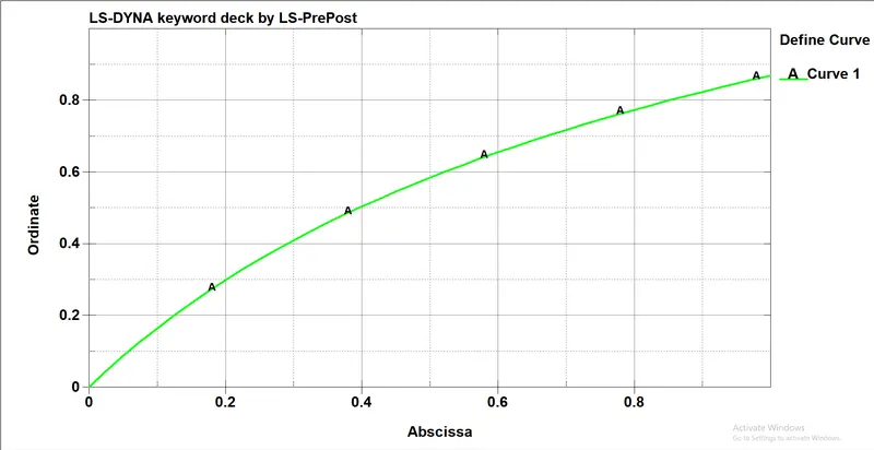
• After defining the curve we need to create the material model.
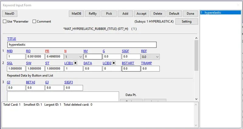
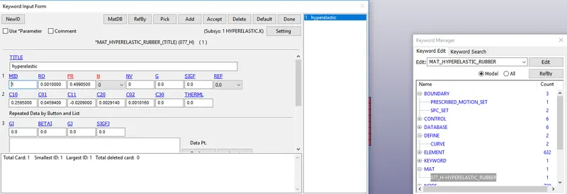
• To create we need to goto MAT and select MAT_77(Hyper_elastic material).
• Here we need to do calibration because there are different parameters to define hyperelastic material.
• To define the hyperelastic card to the model we need to give the variables for hyperelastic materials.
• To calculate them we need to run the simulations with N1, N2, N3 where we will get the stretch ratio and the true stress values.
• From that, we need to correlate with the material curve and stimulated stretch ratio and the true stress values by changing the variablesN1, N2, N3 in the material card.

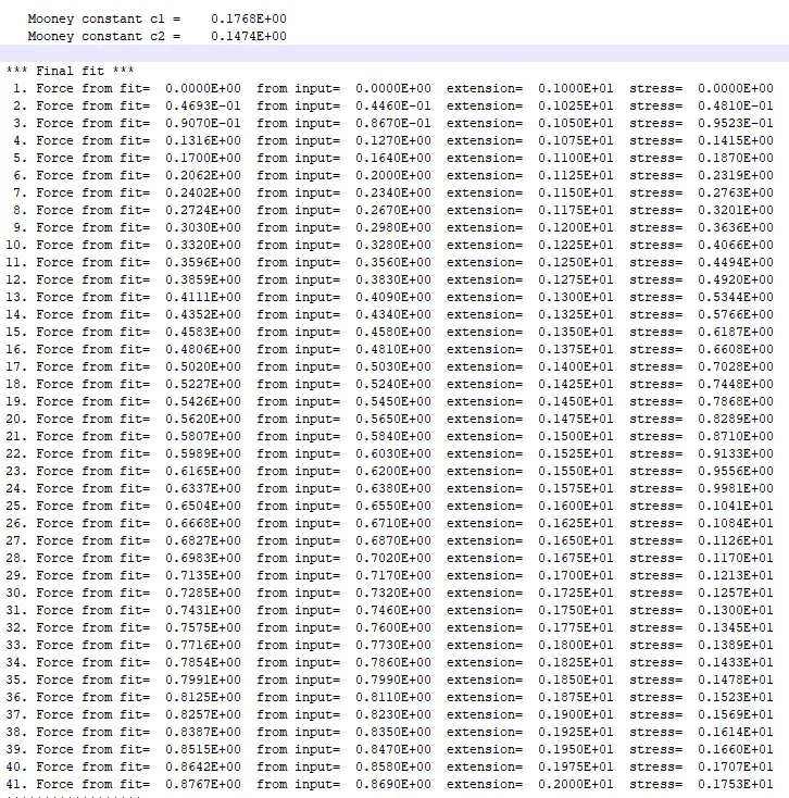
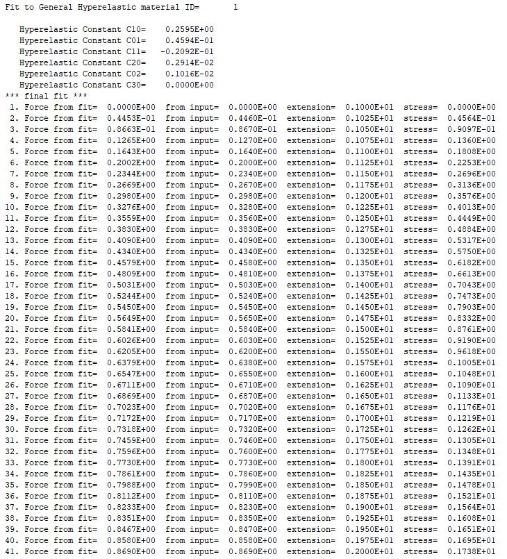
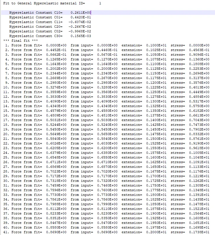
• Where here extension is stretch and stress is true stress.
• To compare we need to convert this to engineering stress and engineering strain.
• True strain=ln(1+engineering strain)
• True stress=engineering stress*exp(true strain) or engineering stress*(1+engineering strain).

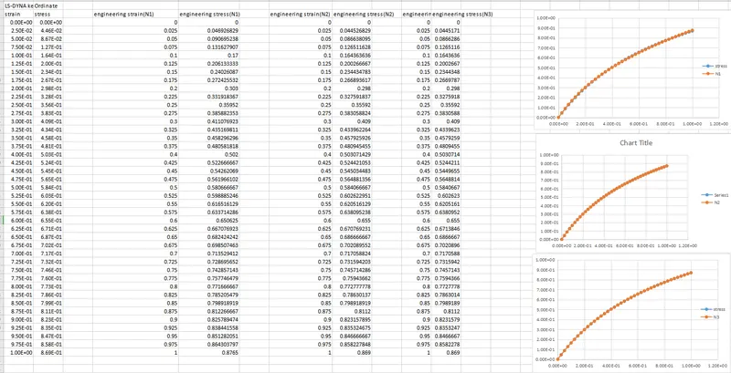
• We can use the values of N2, N3 are exact replica of the experimental values of stress and strain.
• N=0 for defining curve constant without actual defining the curve (C10,C01,C11,C20,C02... etc)
• N=1 for defining curve with Mooney-Rivlin constant.
• N=2 and n=3 for Ogden constant.
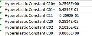
• We can choose any values of n2,n3 like c10,c01,c11,c20,c30,c02,and give that in the material data where we should keep n=0.
• Here I am considering the N=2 values where those values are
• 
• 
• Then set to the part and run the model.
• RESULTS:-

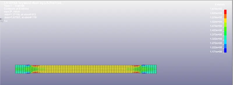
• Here the maximum stress attained by the model is 1.677 N/mm^2

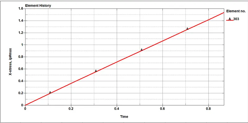
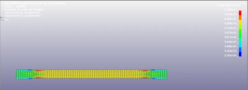
• The maximum strain attained by the component is 6.785e-01

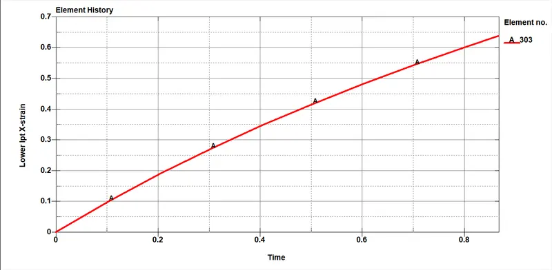
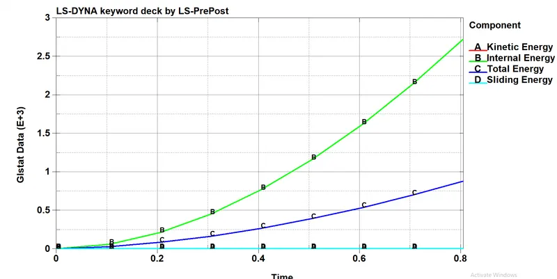
• Where here kinetic energy is neutral because there is very little displacement so that the kinetic energy is constant.
• Here we are going to plot a graph of x-strain and x- stress which is true stress vs true strain.
• Now we need to cross plot the above two graphs.
• To cross plot we need to save the two files and the go-to post-processing then select XY plot.
• Then load the file and cross plot the graph.

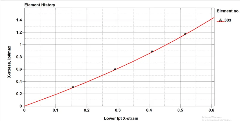
• Now we need to correlate the material data and graph after stimulating.

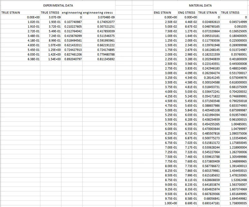
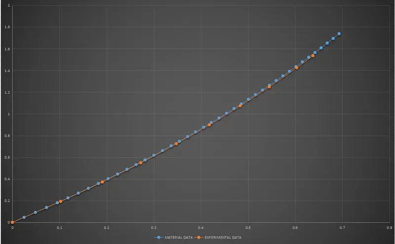
• There is an exact correlation between the material data and experimental data.
• But due to some nonlinearities, the is some deviation this is accepted.

CONCLUSION:-

• Understood how to extract material curve data from the experimental value.
• Understood how to import material curve to the material card in the solver.
• Understood how to correlate the experimental data with material curve data.