Mixing Tee Analysis of a Pipe

Aim-

• to set up steady-state simulations to compare the mixing effectiveness when hot inlet temperature is 36⁰C & the Cold inlet is at 19⁰
• Use the k-epsilon and k-omega SST model for the first case and based on your judgment use the more suitable model for further cases
• Simulate each case for given velocity and momentum ratio
• compare the from the 2 cases about Cell count, Average outlet temperature, Number of iterations for convergence
• Following is required as output data-

1. Velocity and temperature contour plots on the cut planes along and across the pipe.
2. Velocity and temperature line plots along and across the length of the pipe.
3. Perform Mesh independent study for any one case.
4. Discuss the effect of length and momentum ratio on results.
5. Lastly, for each simulation, show the convergence plot

Objective-

• Understand and define problem solution for each case
• Problem Setup-

1. Open Ansys workbench→ Fluent
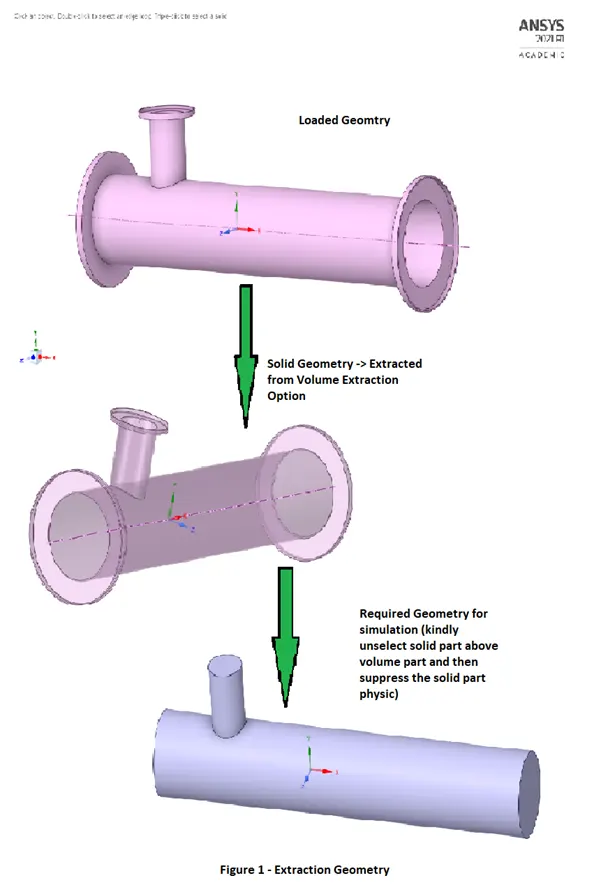
2. From Fluent Setup Tab → Geometry (i.e., Space Claim) → Load Geometry (File Menu →Open) → Extract the geometry as shown in Figure 1
3. Mesh Setup → Insert → Named Selection → Rename and select the Part/Face/Edge accordingly
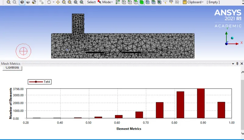
4. Check Mesh Independencies from following flow (Consider Quality Metrics & Element vs Nodes) Any one solution case can be taken in-consideration
5. Meshing-1 → Default mesh setting → Generate mesh
6. Meshing-2 → Element size – 0.004 from default 0.01029 → Generate Mesh
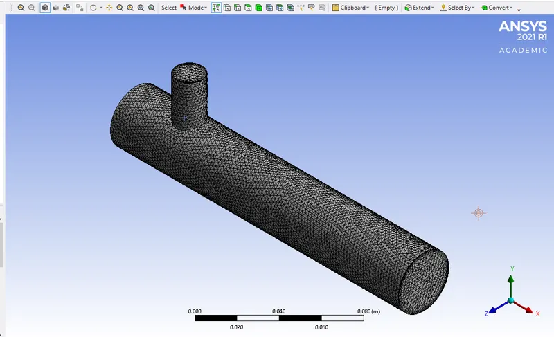
7. Meshing-2 → Element size – 0.002 with Mesh Inflation near Walls → Generate Mesh
8. Note – While creating inflation if one considers Body as selection 1 then selection 2 must be Face and similarly if Face as selection 1 then selection 2 must be Edge
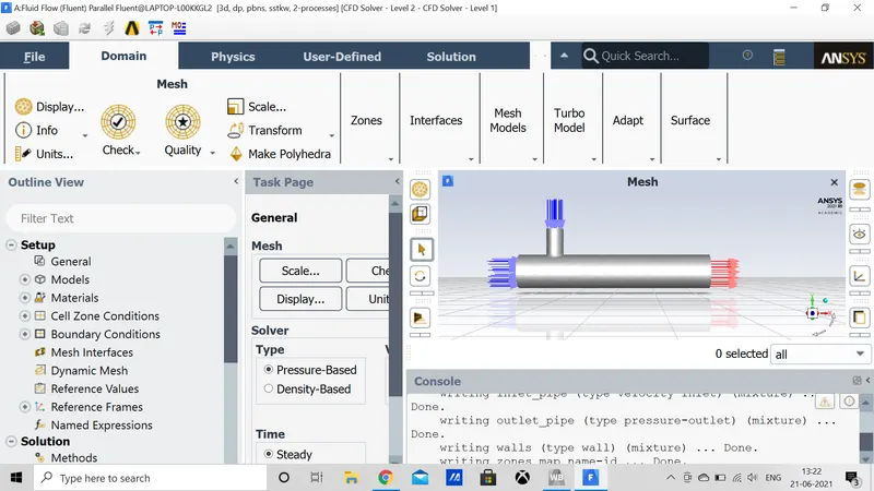
9. Open Fluent Setup → Double Precision → Series run → In Ansys Academic parallel run is not possible due Licensing Issue but can run in Cracked version
10. In Solution Setup – follow the flow below –
11. General → Check Scale (If required change) → Units – From kelvin to Celsius → Check Mesh → Steady state → Absolute
12. Model → Energy equation → Setup-1 - K-epsilon (Change Standard to Realizable) → Setup-2 – K-omega-SST method.
13. Materials → Default (Fluid-Air & Solid-Aluminum) → If required change by adding from fluent material database.
14. Cell Zone Condition → For specific Name Selection change the material here itself otherwise one has reset everything.
15. Boundary Condition → Setup Changes according to the C
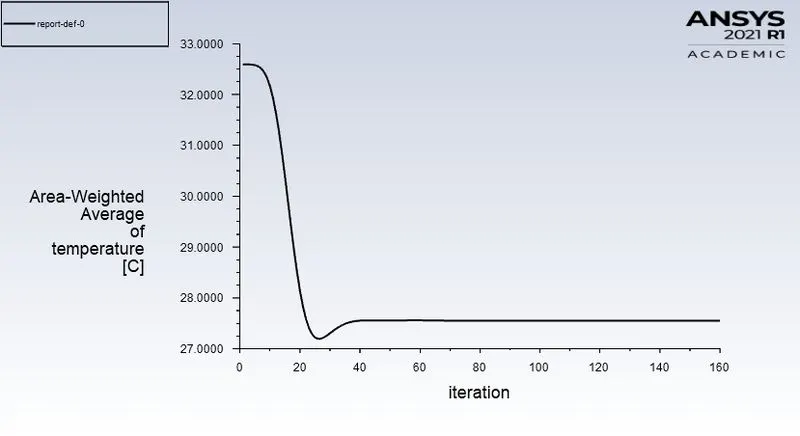
16. Solution → Definitions →New → Surface Report → Area-Weighted Average/Also Standard Deviation → Temperature/velocity → Surface Selection (Pipe Outlet) → Report File & Print Console
17. Hybrid Initialize (Patch not required) → Run Calculation → iteration as per problem requirement → Time step – 0.5 sec or 1 sec.

• Compare Cell Count, Avg, Temp and No of iteration to converge
• Validate results from contour plot and line plot for temperature & velocity respectively.
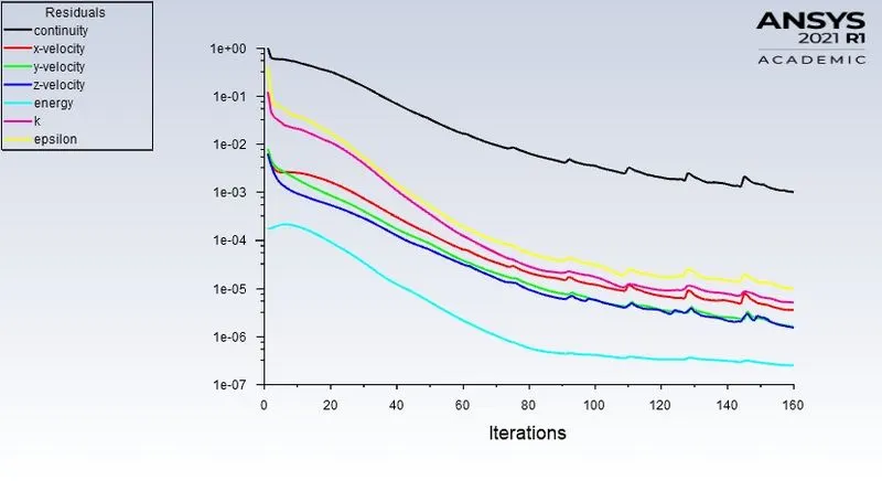
• From Convergence Plot, verify that the results are fully converged after running numerous iters.
• Study the effect of length and momentum ratio on results of each case.

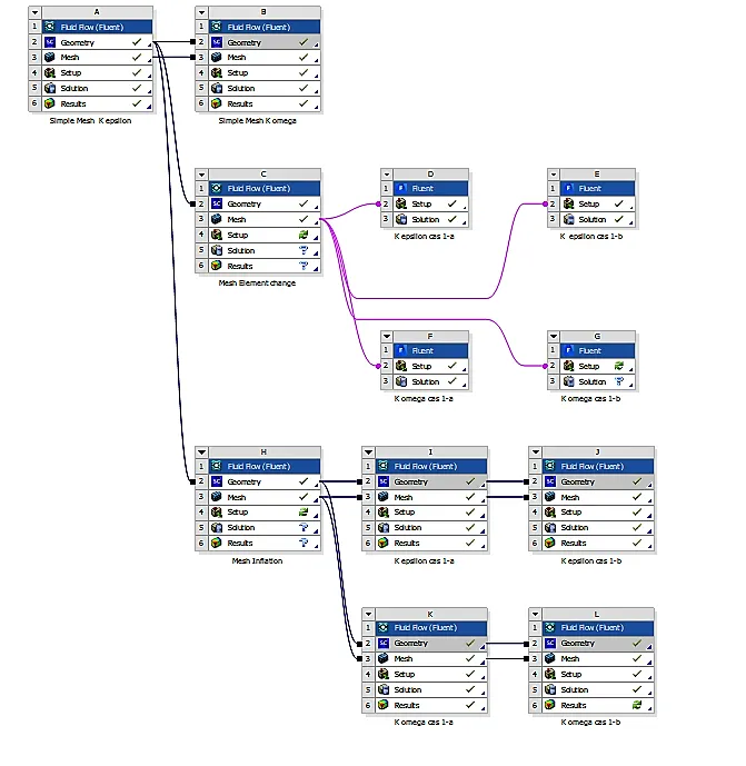
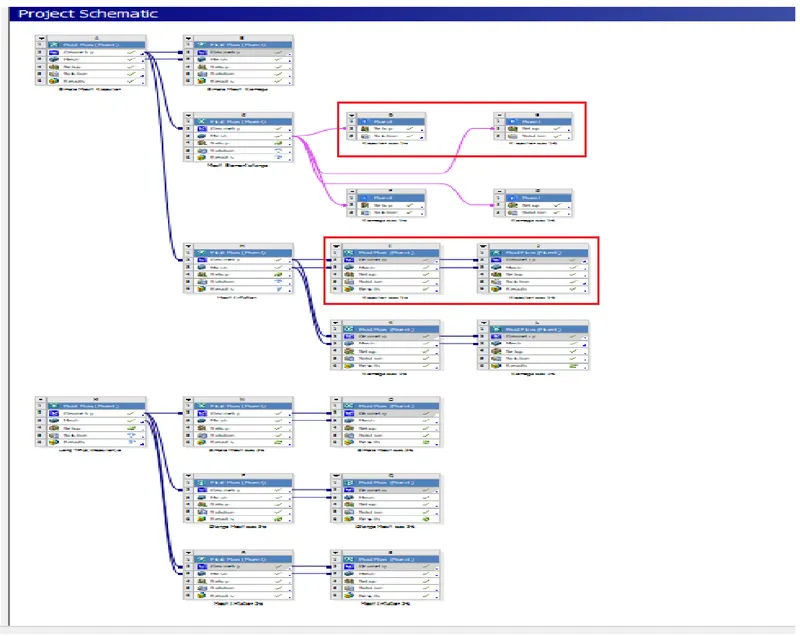
Ansys Project Schematic -

For Short mixing T-pipe similar can be followed in-case of Long T-pipe

Theory -

K-epsilon –

• In simulation 1 we choose, K-epsilon turbulent model as it’s the most common model used in CFD to simulate mean flow characteristics for turbulent conditions.
• It’s a 2-equation model that give a description of turbulence by means of 2-transport equation (PDEs).
• We can tell that First Transport variable is turbulent kinetic energy (e) and 2^nd transport variable is rate of dissipation of turbulent kinetic energy
• K-epsilon focuses on the mechanism that affect the turbulent kinetic energy.

K-Omega –

• K-omega SST turbulence model is a 2 equation Eddy-Viscosity Model that is mainly used in aerodynamic applications.
• It is a hybrid model combining Wilcox K-omega and K-epsilon models.
• In simulation, we see that near the walls Wilcox model gets activated and the K-epsilon model is for free stream.
• This ensures that appropriate model is utilized through flow field.

Comparison –

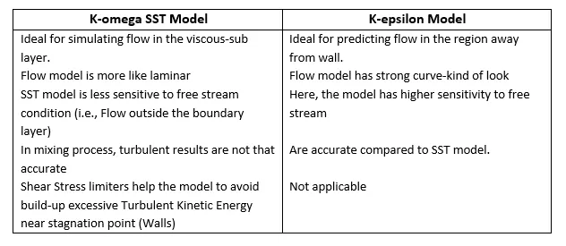
Hence, for further simulation in Long T-pipe I am using K-epsilon model as we are not instructed to find the convergence near the walls specifically.

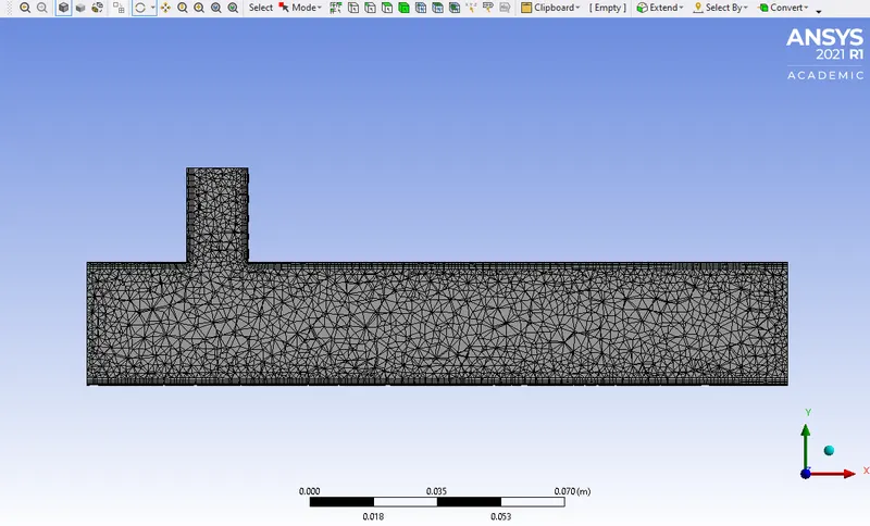
Simple Mesh Generated -

All the settings are set default-

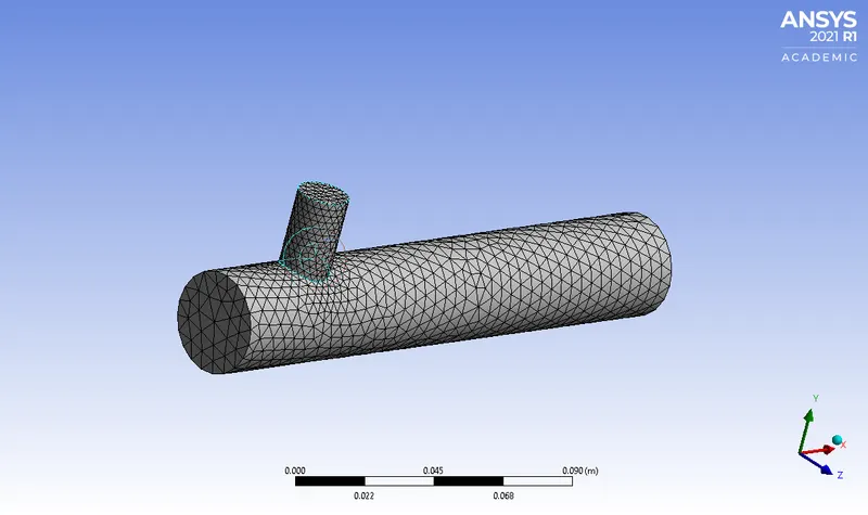
Cut half Pipe Mesh-

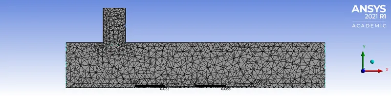
Quality `->`Element Metrics

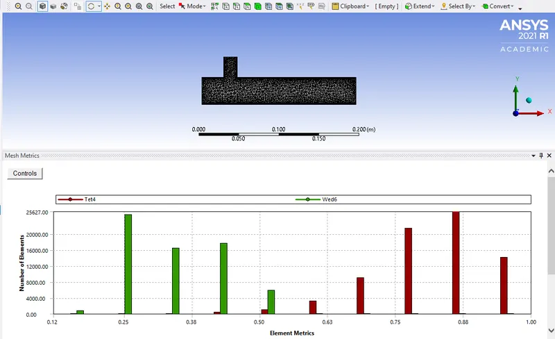
Mesh with inflation -

Cut half Pipe Mesh-

Quality `->`Element Metrics

Case 1-a - Cool_inlet =12 m/s

Hot_inlet = 3 m/s

Hot_outlet = pressure gauge = 1 atm

Cool_inlet_Temperature = 19*C

Hot_inlet_Temperature = 36*C

Convergence Plot -

Area-Weighted Average of Temperature at Oullet -

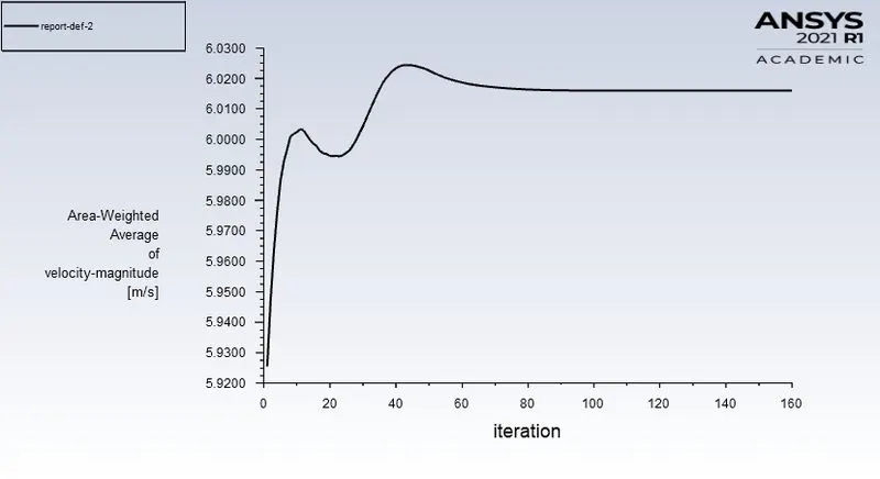
Area-Weighted Average of Velocity at Oullet -

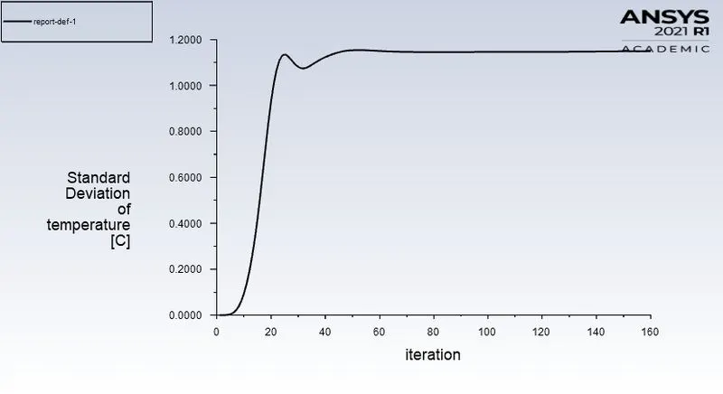
Standard Deviation of Temperature at Oullet -

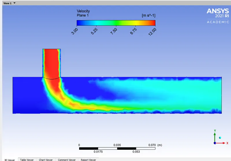
Velocity Contour along the length of Pipe -

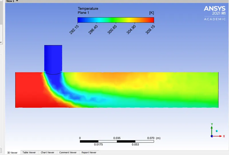
Temperature Contour along the length of Pipe -

Streamline Velocity Contour along the length of Pipe -

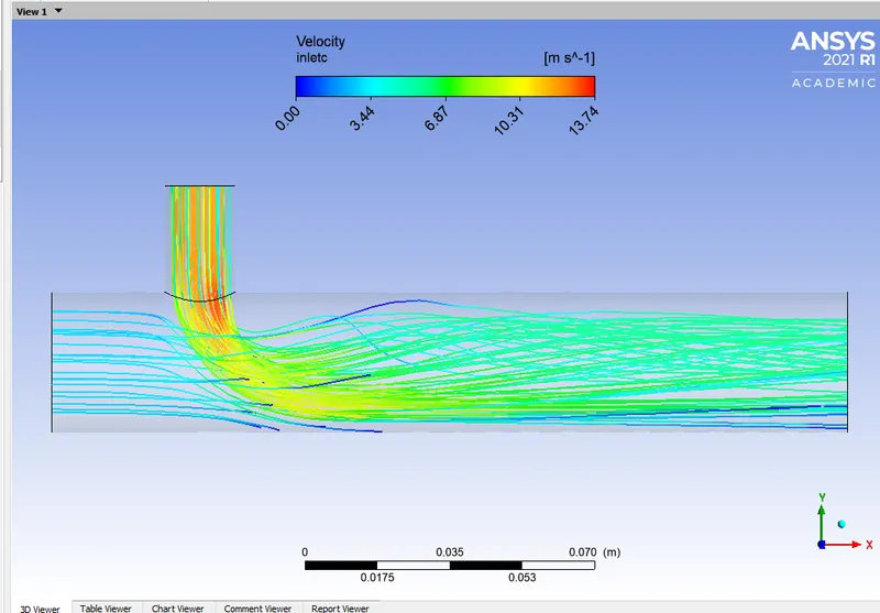
Streamline Temperature Contour along the length of Pipe -

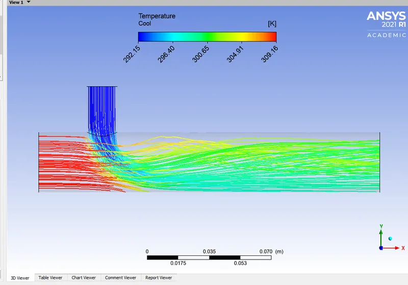
Case 1-b - Cool_inlet =6 m/s

Hot_inlet = 3 m/s

Hot_outlet = pressure gauge = 1 atm

Cool_inlet_Temperature = 19*C

Hot_inlet_Temperature = 36*C

Convergence Plot -

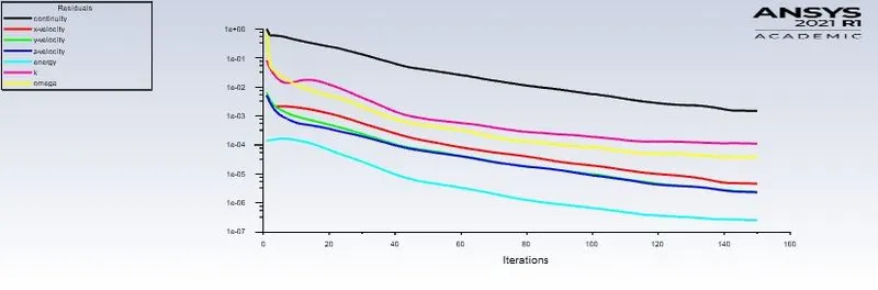
Area-Weighted Average of Temperature at Oullet -

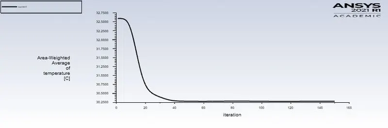
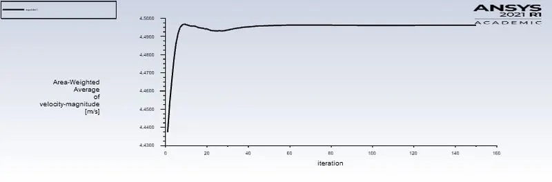
Area-Weighted Average of Velocity at Oullet -

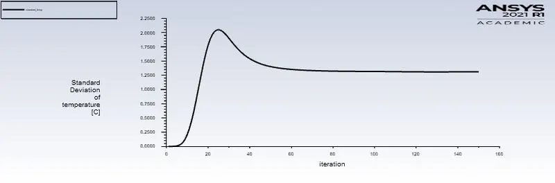
Standard Deviation of Temperature at Oullet -

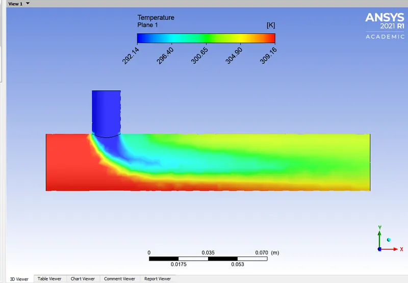
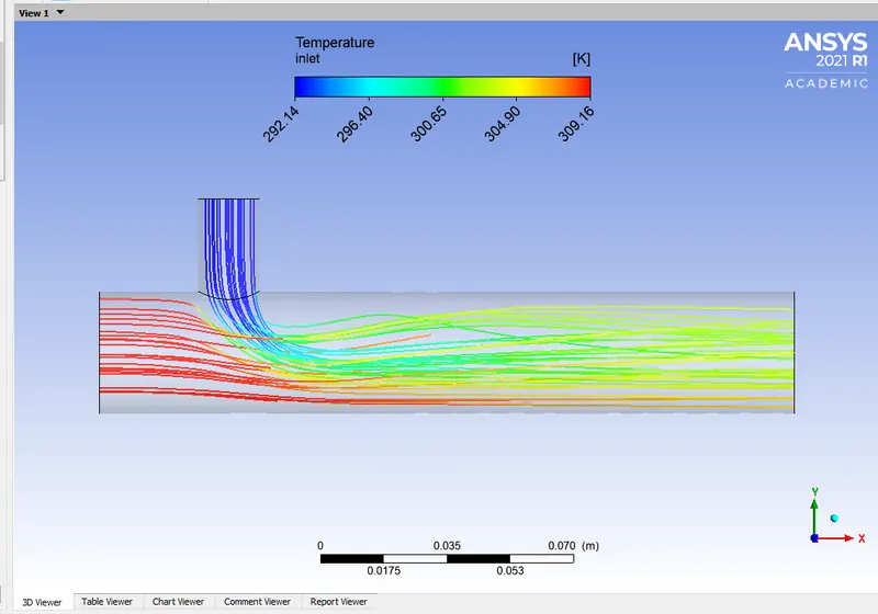
Temperature Contour along the length of Pipe -

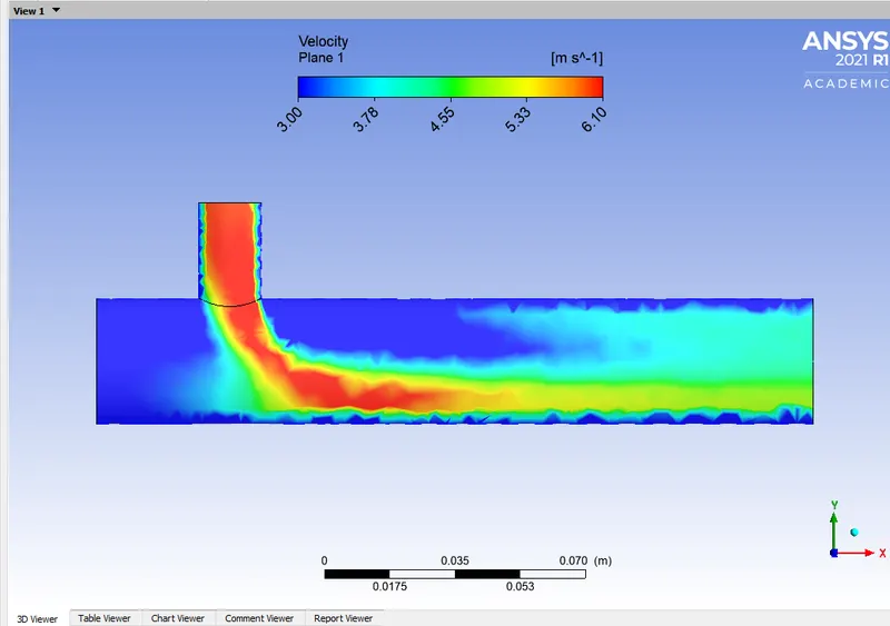
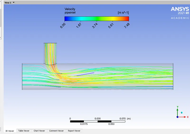
Velocity Contour along the length of Pipe -

Streamline Temperature Contour along the length of Pipe -

Streamline Velocity Contour along the length of Pipe -

Output Table 1 -

Short T-Mixing Pipe

Scheme - K-epsilon

Case 1-a

Momentum Ratio = 4
Element Size (Mesh)	Cell Count (No. of Nodes & No. of Elements)	Avg. Temperature @ Output in °C	Avg. Velocity @Output In m/s	Standard Deviation Temperature In °C	Iterations
Default (1.0219e-003)	2808 / 12632	27.5504	6.0160	1.1499	160

Scheme - K-omega (SST-Method)

Case 1-b

Momentum Ratio = 2
Element Size (Mesh)	Cell Count (No. of Nodes & No. of Elements)	Avg. Temperature @ Output	Avg. Velocity @Output	Standard Deviation Temperature	Iterations
Default (1.0219e-003)	2808 / 12632	30.280	4.496	1.309	180

From the above output tables, we achieve to a conclusion that only and if specified to find the convergence of fluid flow near the walls of pipe then we can use hybrid scheme - K-omega (SST-model) else we can stick to K-epsilon model. Where in we tend to observe the free stream flow (Visicous Sub-Layer) throughout the pipe.

Camparison b/w all cases

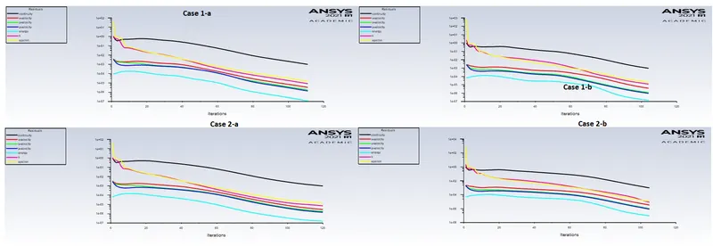
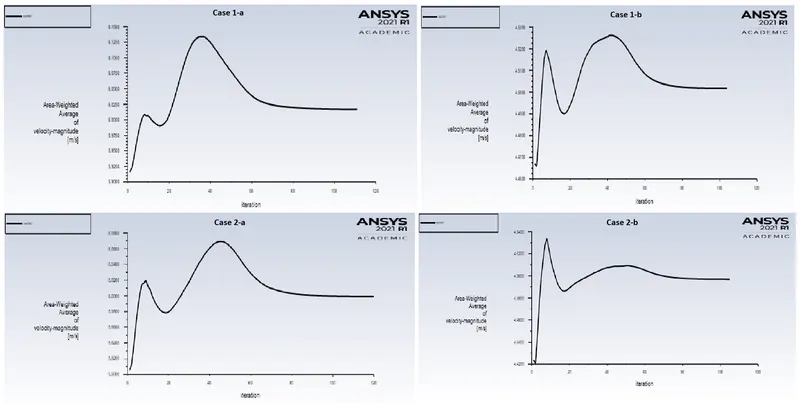
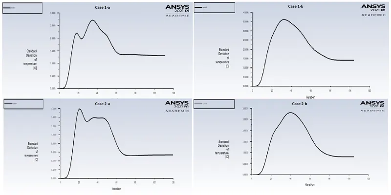
Convergence Plot -

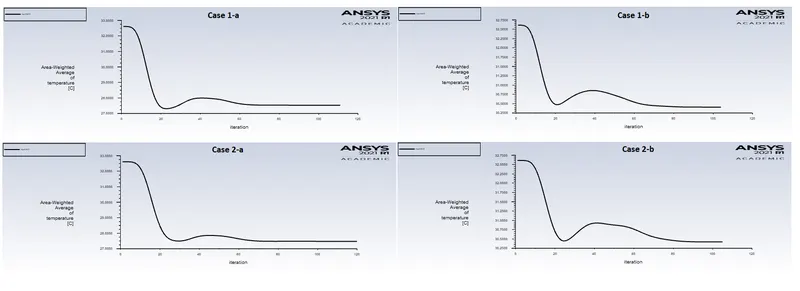
Average Weighted Temperature along the length of Pipe -

Average Weigthed Velocity along the length of Pipe -

Standard Deviation Temperature along the length of Pipe -

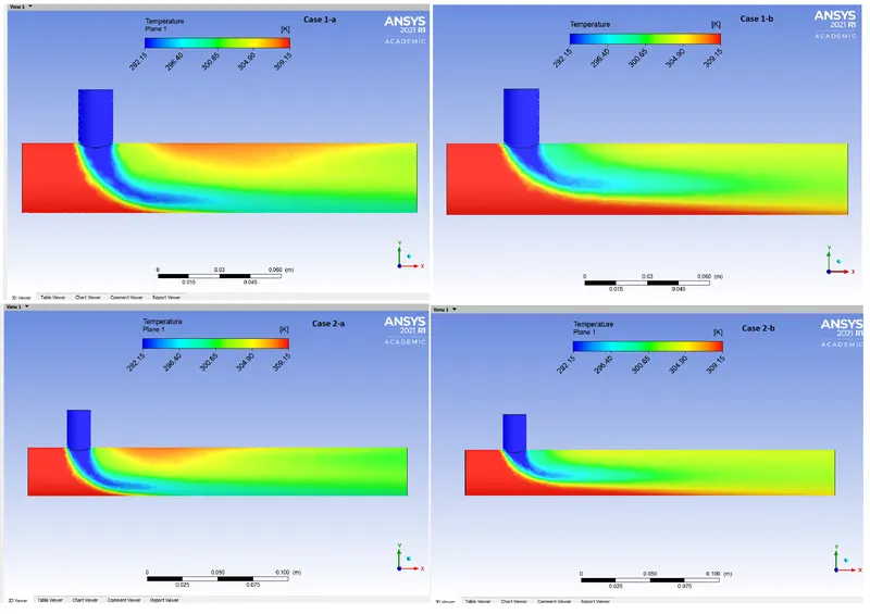
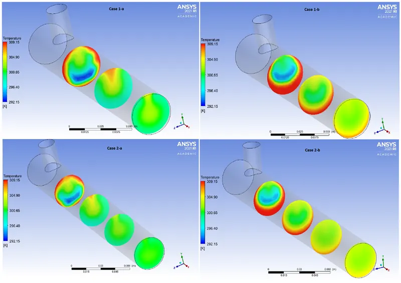
Temperature Contour along the length of Pipe -

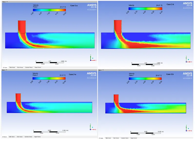
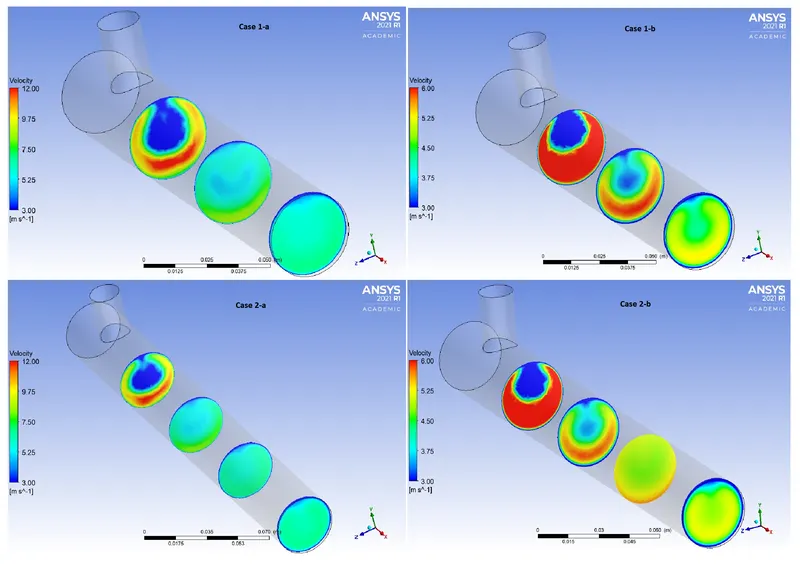
Velocity Contour along the length of Pipe -

Temperature Contour across the Pipe -

Velocity Contour across the Pipe -

_________________________________________________________________________________________________________

Mesh Independent Study

Mesh indepent test allows the user to create quality mesh refinement and determine the dependencies of same on simulation results. This type of study allows the user to define a preicise results.

Problem Setup -

Here the objective, is compare results with different mesh sizing this can be obtained by running various simulations mesh change and in bid to pass the Mesh Idenpendence results the user learns the importance of meshing in a design geometry and change of which implies to preicison simulation results.

In our Case, we run three mesh changes and simulations for each setup case for validation of study

Output Table 2 -

Short Pipe -

Momentum Ratio = 4
Element Size (Mesh)	Cell Count (No. of Nodes & No. of Elements)	Avg. Temperature @ Output in °C	Avg. Velocity @Output In m/s	Standard Deviation Temperature In °C	Iterations
Default (1.0219e-002)	2808 / 12632	27.5504	6.0160	1.1499	160
0.004	4742 / 22040	27.5706	6.0126	0.9921	134
Inflation 0.002	49107 / 140075	27.5260	6.0165	1.2109	120

Momentum Ratio = 2
Element Size (Mesh)	Cell Count (No. of Nodes & No. of Elements)	Avg. Temperature @ Output	Avg. Velocity @Output	Standard Deviation Temperature	Iterations
Default (1.0219e-003)	2808 / 12632	30.280	4.496	1.309	180
0.004	4742 / 22040	30.322	4.495	1.507	160
Inflation 0.002	49107 / 140075	20.407	4.501	1.401	110

Long Pipe -

Momentum Ratio = 4
Element Size (Mesh)	Cell Count (No. of Nodes & No. of Elements)	Avg. Temperature @ Output in °C	Avg. Velocity @Output In m/s	Standard Deviation Temperature In °C	Iterations
Default (1.0219e-002)	3477 / 15610	27.485	6.000	0.782	160
0.004	6236 / 29044	27.509	5.998	0.6167	131
Inflation 0.002	86269 / 186702	27.477	5.999	0.539	120

Momentum Ratio = 2
Element Size (Mesh)	Cell Count (No. of Nodes & No. of Elements)	Avg. Temperature @ Output	Avg. Velocity @Output	Standard Deviation Temperature	Iterations
Default (1.0219e-003)	3477 / 15610	30.280	4.496	1.309	180
0.004	6236 / 29044	30.322	4.495	1.507	140
Inflation 0.002	86269 / 186702	30.422	4.496	0.811	110

Conclusion -

• We can notice that diffusion flow allow gives better mixing of two-fluid, when the length of T-mixing increases.
• From the Output Table 2, higher momentum ratio provides better mixing of hot and cold fluid stream at outlet.
• In order to save simulation time and runs one can flow this –
• (1) Let your first simulation on fluid domain use coarse mesh (default), which in turn returns the user to have an initial overview analysis of convergence occurring at faster pace.
• (2) Repeat the same with gradual increase in element size / coarse mesh only. This leads to understanding of how increase in mesh element increase simulation time.
• (3) After successfully completion and understanding of above simulation. The user can perform refinement of mesh quality and obtain precision results.
• K-epsilon model predicts flow virtually far from the boundaries (Wall).
• K-omega SST model predicts the flow near the boundaries (Wall).
• Since, we are analysing Turbulent Flow Model away from wall. We tend to use K-epsilon flow model.
• Finally, in above cases. It is very important to use short T-mixing pipe with momentum ratio = 4 to obtain precise results but one has to consider the diffusion of flow along the length of T-mixing.
• With the same momentum the diffusion rate with be higher in long T-mixing pipe.