External flow simulation over an Ahmed body in Wind Tunnel

Aim – To simulate external flow over an Ahmed body using steady-state, density-based solver and performing grid independency test respectively.

Objective –

1. Briefing about Ahmed’s body and its significance
2. Explain the reason for the negative pressure in the wake region.
3. Explain the significance of the point of separation.

Theory –

The flow over road vehicles under normal operating conditions is principally turbulent which is characterized by large-scale operation and recirculation regions, complex wake flows, long trailing vortices and interaction of boundary layer flow on vehicle and ground.

In aerodynamics flow around a vehicle, it’s a 3-D flow and the design will have an influence on principle features like

• Shape of the vehicle
• Aerodynamic drag
• Fuel consumption
• Noise production
• Road handling

By using wind tunnel testing, designers have an understanding on airflow around vehicle dynamics through extensive experiments. But wind tunnel testing for every prototype is a time-consuming and costly process. In order to reduce time, it’s necessary to use simplified computational technique and adopt a model to describe mean effect of turbulence.

Unfortunately, a simple model of turbulence often fails to calculate the flow properly especially the position of flow separation. To overcome the problem. S R Ahmed in 1984 described an Ahmed body with standard results to test various types of challenges and turbulence models.

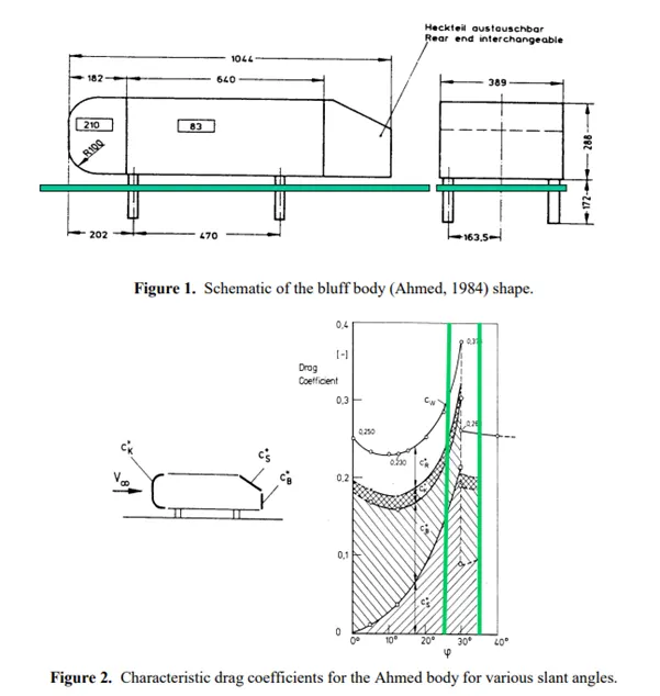
Ahmed body is a bluff body whose shape is simple enough to model while maintaining certain car-like features. Ahmed body is widely used in vehicle aerodynamics to validate numerical model with experimental data from wind tunnel testing available for the same. Once the numerical model is validated its used to design new models of ground vehicles.

Coefficient of Drag -

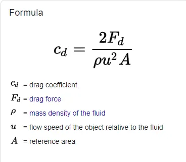
In fluid dynamics, the drag coefficient (commonly denoted as: C_{d } , C_x or C_{w }) is a dimensionless quantity that is used to quantify the drag or resistance of an object in a fluid environment, such as air or water. It is used in the drag equation in which a lower drag coefficient indicates the object will have less aerodynamic or hydrodynamic drag. The drag coefficient is always associated with a particular surface area
The drag coefficient of any object comprises the effects of the two basic contributors to fluid dynamic drag: skin friction and form drag. The drag coefficient of a lifting airfoiled or hydrofoil also includes the effects of lift-induced drag. The drag coefficient of a complete structure such as an aircraft also includes the effects of interference drag.

Coefficient of Lift –

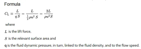
The lift coefficient () is a dimensionless coefficient that relates the lift generated by a lifting body to the fluid density around the body, the fluid velocity and an associated reference area. A lifting body is a foil or a complete foil-bearing body such as a fixed-wing aircraft. C_L is a function of the angle of the body to the flow, its Reynolds number and its Mach number. The section lift coefficient c_l refers to the dynamic lift characteristics of a two-dimensional foil section, with the reference area replaced by the foil chord.

Procedure –

Problem Setup –

• (1) Geometry

Files → Space Claim Options → Units

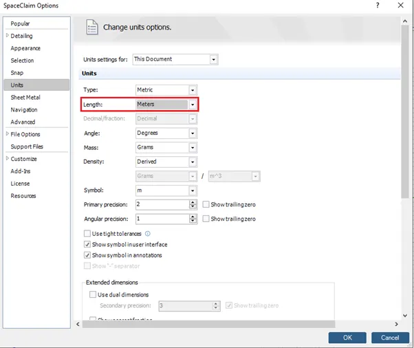
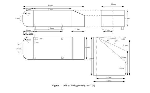
Create a geometry in Space Claim with following dimensions,

• Mesh Generation –

Right Click → Insert → Named Selection, As follows

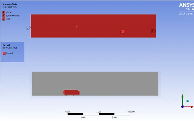
Recommended, generate mesh with default settings and check the simulation for only first case. If not sure how mesh element sizing and other mesh techniques are used to enhance the quality of mesh.

Mesh Baseline –

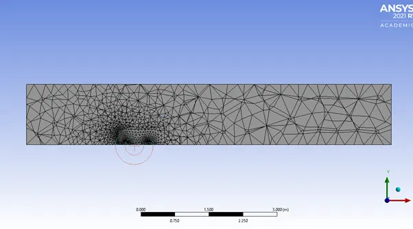
Mesh Details –

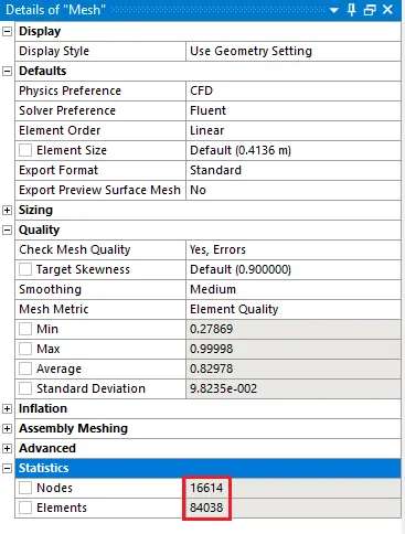
Mesh Quality–

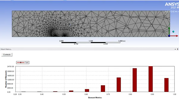
• Mesh Setting for refinements –

Right Click → Insert → Methods,

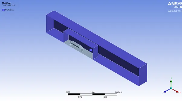
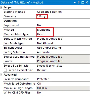
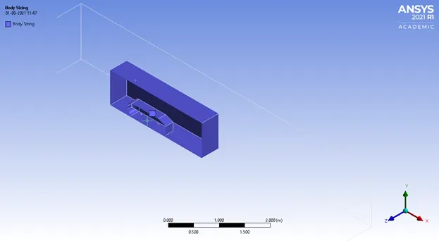
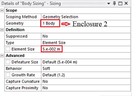
Right Click → Insert → Body Sizing,

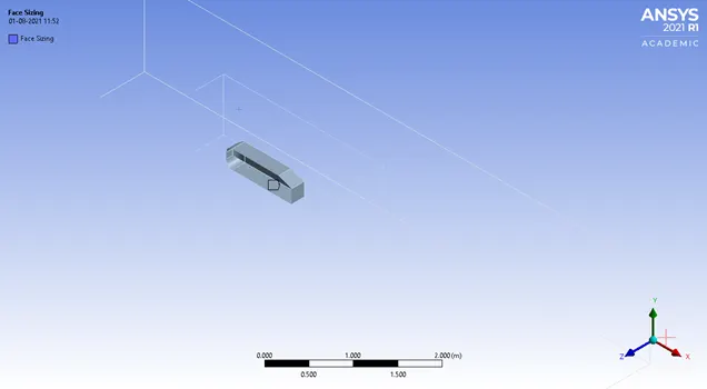
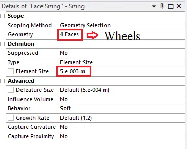
Right Click → Insert → Face Sizing,

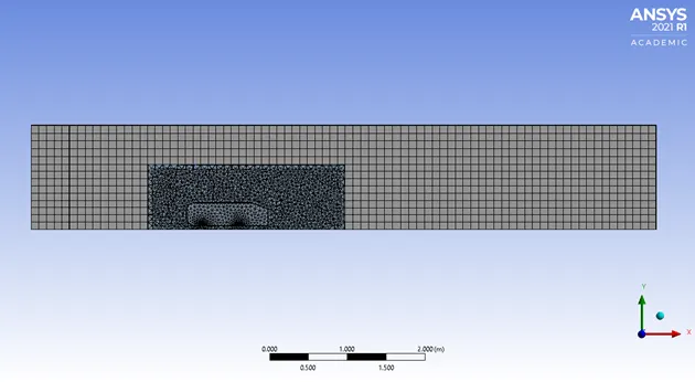
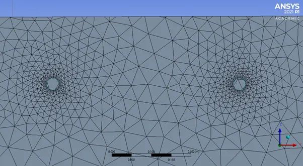
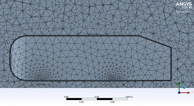
Mesh Refinement 1 –

Mesh Details –

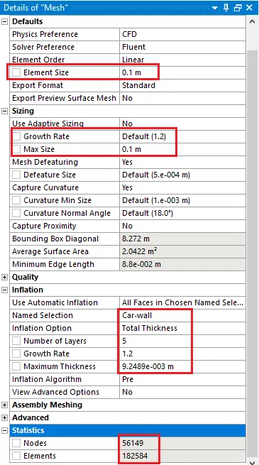
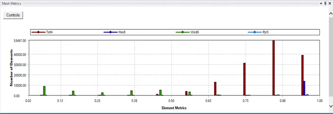
Mesh Quality –

Inflation (Car Wall) → First Layer Thickness Calculation

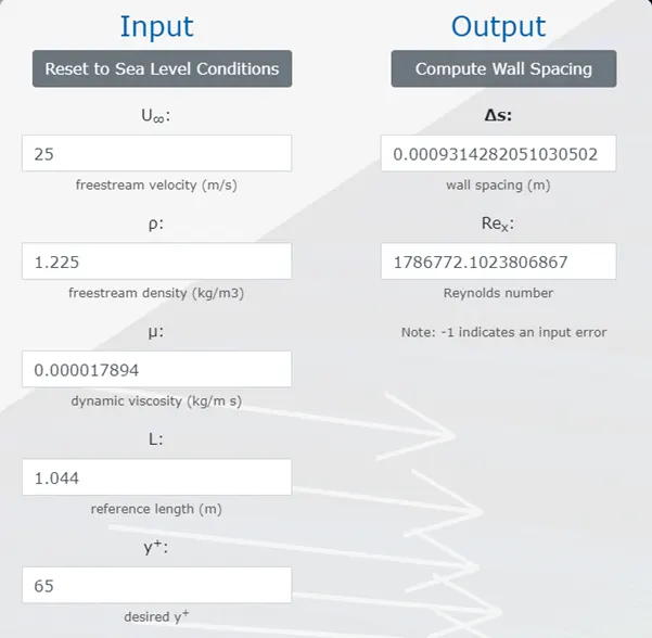
Mesh Refinement 2 –

Inflation (Car Wall) → First Layer Thickness Calculation

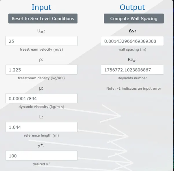
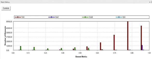
Mesh Quality –

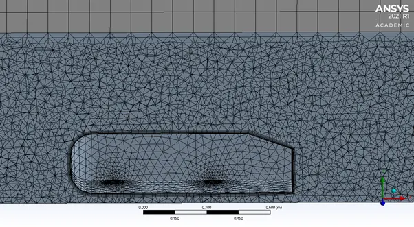
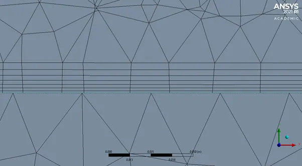
Mesh Details –

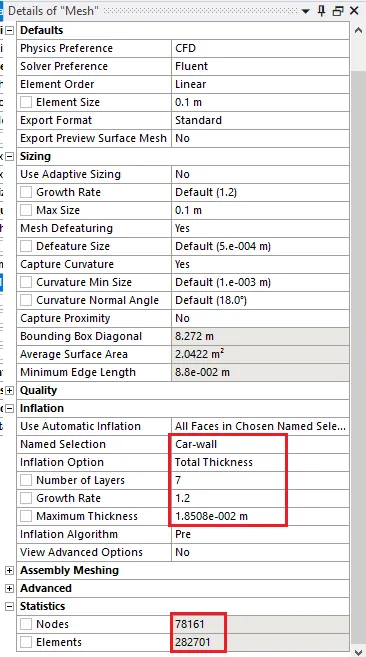
Mesh Refinement 3 –

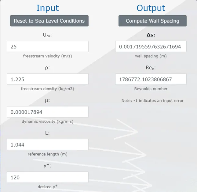
Inflation (Car Wall) → First Layer Thickness Calculation

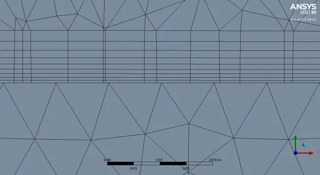
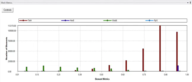
Mesh Quality –

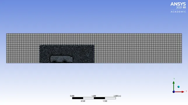
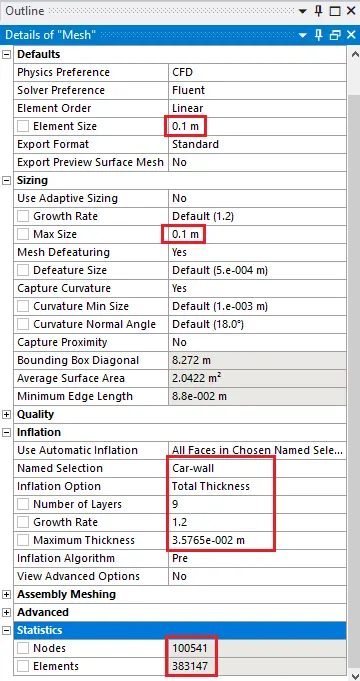
Mesh Details –

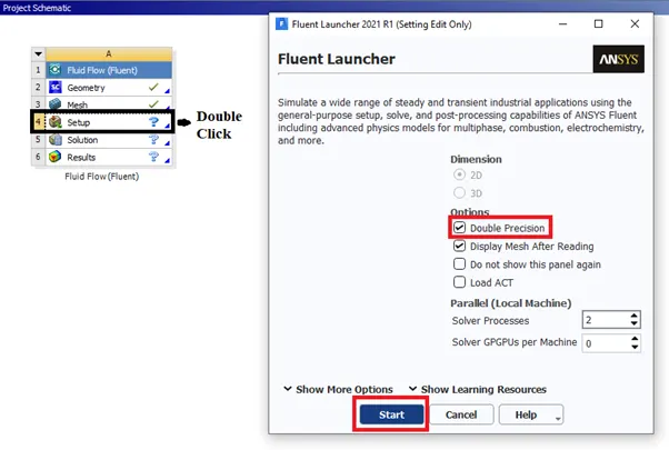
• Fluent Setup –

• Solution Setup -

1. General → Solver → Density-based → Time→ Steady State
2. Model → Energy → On
3. Models → Viscous → K-epsilon → Standard Model & Wall Function
4. Material → Fluid → Add New → Fluent Database → User-Material (In our case user-material has Density=1 kg/m^3 & Viscosity=0.02 Kg/m-s)
5. Cell Zone Conditions → fff_surface → Fluid → User-material
6. Boundary Conditions

• Intel (Velocity= User-defined/ 25m/s)
• Outlet (Gauss Pressure=1 atm)
• Car-wall → Wall Motion → Stationary → Shear Condition → No Slip
• Symmetry-wall → Symmetry boundary

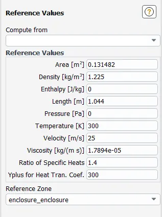
1. Reference Values →

1. Method → Scheme → Simple
2. Results → Create → Line → Point and Normal
3. Solution → Definition →

• Force Report → Lift → Lift Coefficient → Field Variable = Car-wall
• Force Report → Drag → Drag Coefficient → Field Variable = Car-wall

1. Initialize Solution → Hybrid
2. Results →

• Create Contour → Velocity → Field Variable = Cut-plane-Z
• Create Contour → Pressure → Field Variable = Car-wall

1. Activities → Create Animation → Solution Animation → Velocity Contour

• Results –

Baseline Experiment Setup –

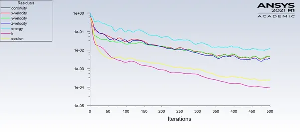
Residual Plot –

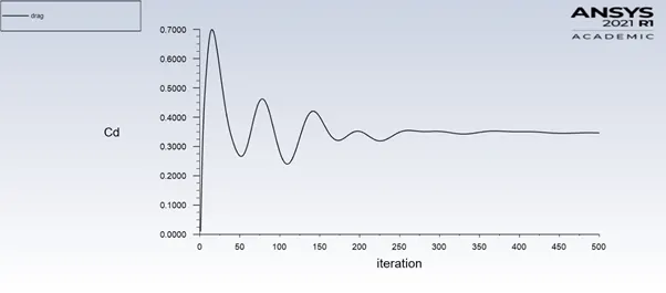
Drag Coefficient Plot –

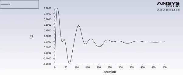
Lift Coefficient Plot –

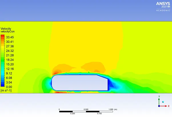
Velocity Contour –

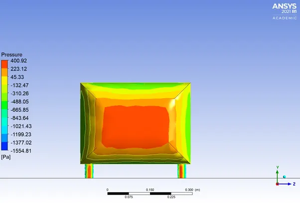
Pressure Contour –

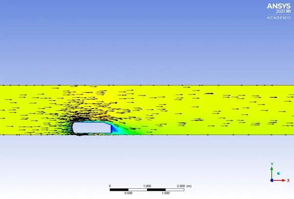
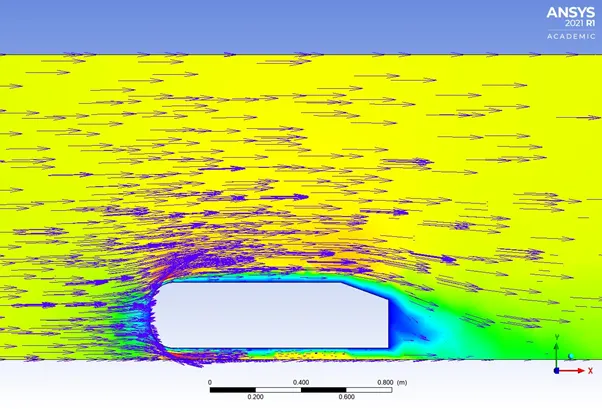
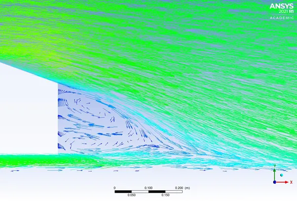
Vector Plot –

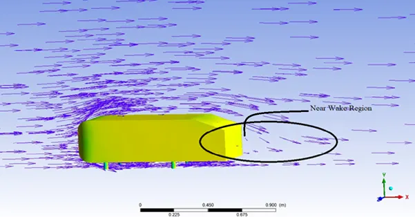
Refinement 1 (5 inflation layer / Y-Plus= 65) Experiment Setup –

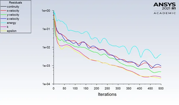
Residual Plot –

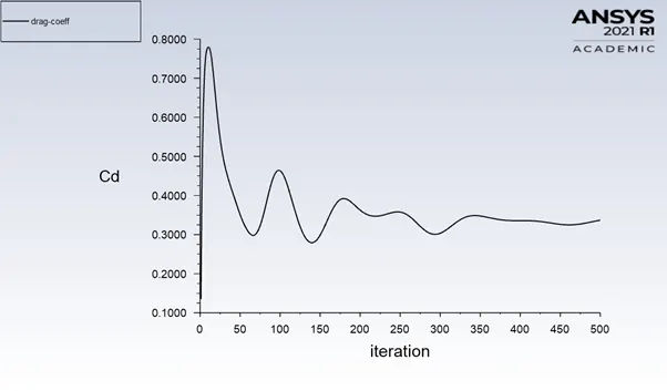
Drag Coefficient Plot –

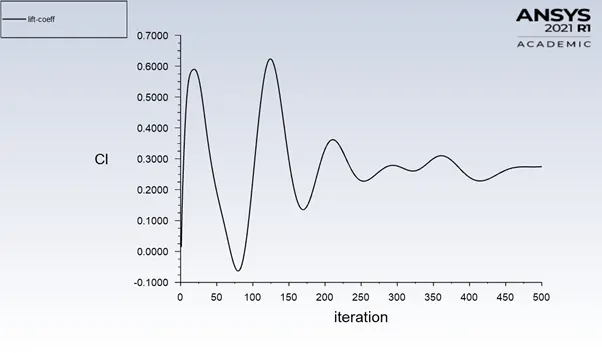
Lift Coefficient Plot –

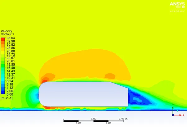
Velocity Contour –

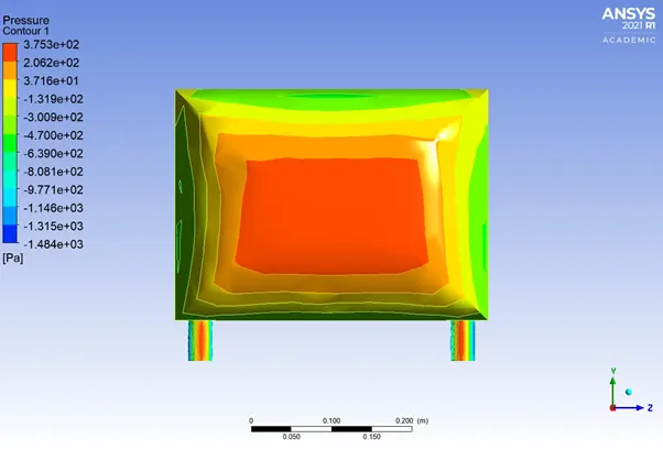
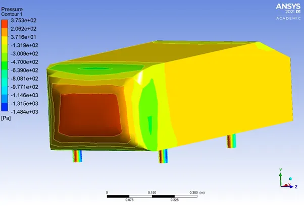
Pressure Contour –

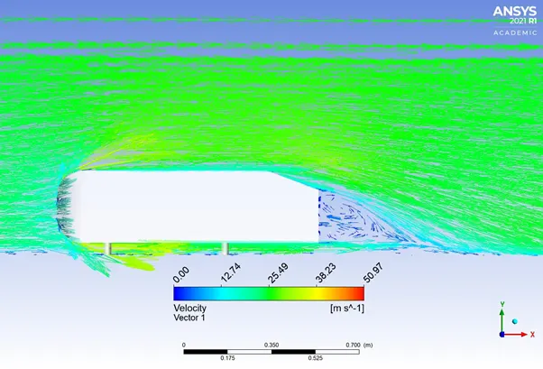
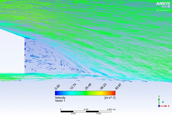
Vector Plot of Wake Region–

Refinement 2 (7 inflation layer / Y-Plus= 100) Experiment Setup –

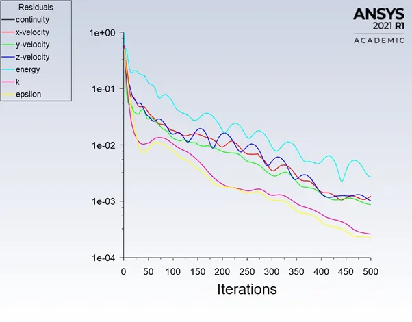
Residual Plot –

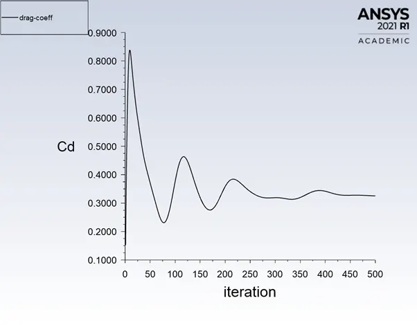
Drag Coefficient Plot –

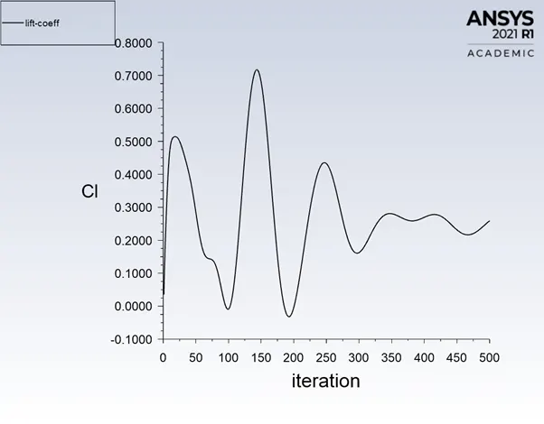
Lift Coefficient Plot –

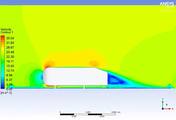
Velocity Contour –

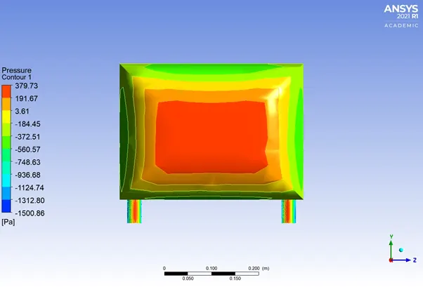
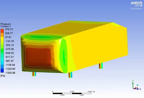
Pressure Contour –

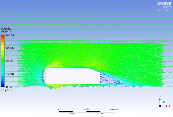
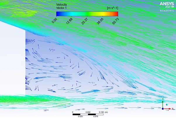
Vector Plot –

Refinement 3 (9 inflation layer / Y-Plus= 120) Experiment Setup –

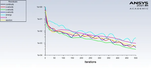
Residual Plot –

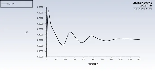
Drag Coefficient Plot –

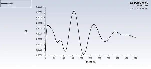
Lift Coefficient Plot –

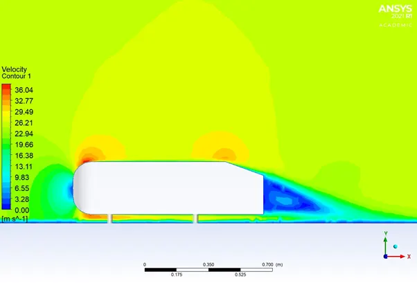
Velocity Contour –

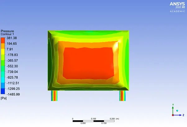
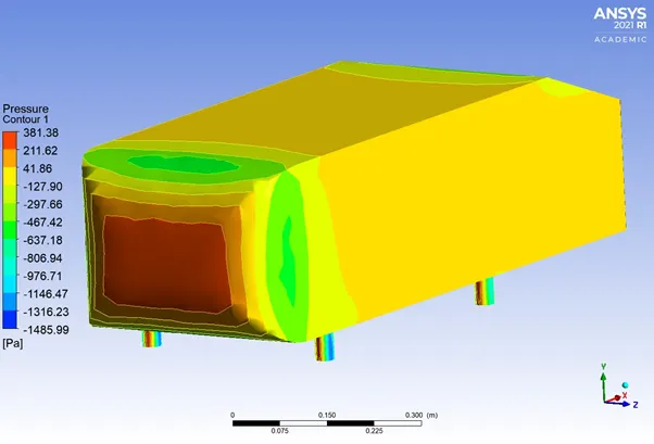
Pressure Contour –

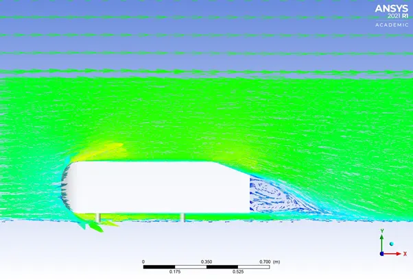
Vector Plot –

Velocity Plot –

• Baseline –

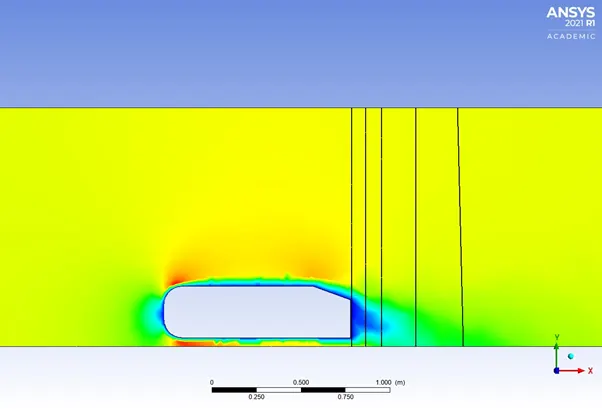
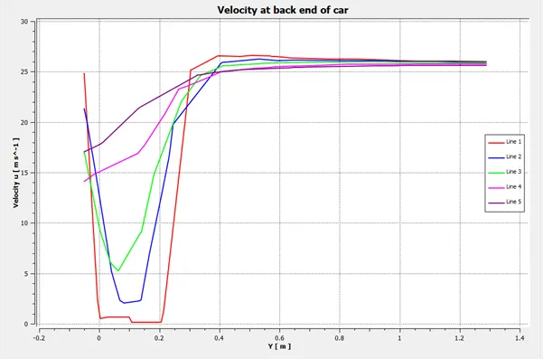
• Line Setup for Refinements –

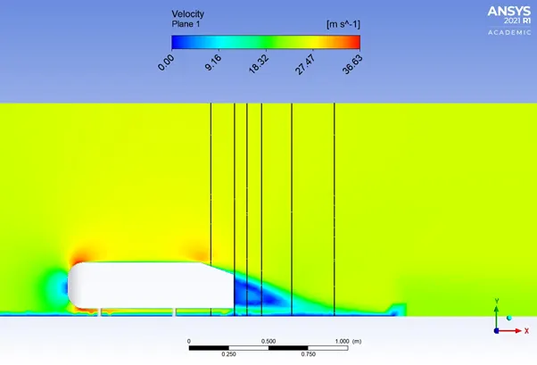
• Refinement 1 –

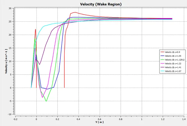
• Refinement 2 –

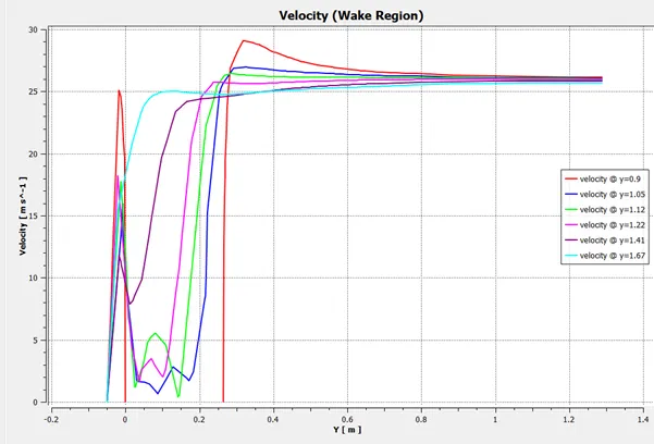
• Refinement 3 –

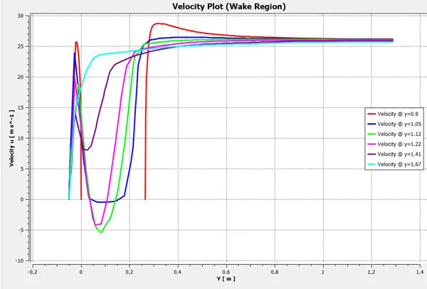
Conclusion –

SL. No	Turbulent Model	Inflation Layer	Elements	Nodes	Coefficient of Drag (Experimental)	Coefficient of Drag (simulation)	Error %	Coefficient of Lift
1	K-e	Baseline	84038	16614	0.279	0.346	24.01	0.197
2	K-e	5	182584	56149	0.279	0.336	20.41	0.274
3	K-e	7	282701	78161	0.279	0.325	16.48	0.259
4	K-e	9	383147	100541	0.279	0.311	11.46	0.264

Inference –

• Simulation results hold a good arrangement with the experimental results for the turbulent model.
• The inflation layer is added advantage to capture the flow near the Ahmed body.
• The cause of slow separation is due negative pressure generated in the boundary layer of flow near the wall of the body.
• We can observe that negative wake region is generated due the pressure difference between a low stream and high stream flow.
• The grid independence test is carried out to demonstrate the variation of the result with respect to accuracy of mesh.
• Good quality of mesh is needed for achieving accurate results.

Negative Pressure in Wake Region –

A high-pressure region is observed infront of Ahmed Body and a drop on pressure is observed when the flow leaves the Ahmed Body at rear end. This can be illustrated using following structure of airfoil flow –

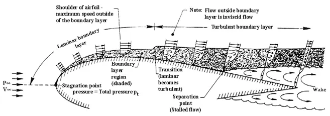
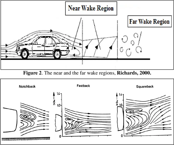
• The detachment of flow at the rear end results in the formation of eddies.
• The region behind Ahmed Body where the flow is unstable is called wake region, where pressure adversely drops.
• At the inlet, fluid flow at velocity 25m/s. when it encounters the Ahmed body in the front, the flow gets stagnated and there is reduction in velocity leading to an increase in pressure.
• The fluid that comes in contact behaves likes a viscous sublayer and this property of flow remains until in contact with the body.
• At slant of Ahmed body, the fluid separates the body and the point of separation is created.
• When the fluid flows over the body, the boundary layer thickness increases.
• The fluid layer adjacent to wall causes surface friction by some kinetic energy.
• This loss of kinetic energy can be recovered by adjacent fluid layer through the momentum exchange process. Thus value of velocity goes on decreasing.
• Along the length od body, at a certain point, a stag may develop when the boundary layer gets separated from the surface. This phenomenon is called boundary layer separation.

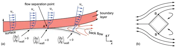
• Near the surface of the solid when the point of separation occurs the fluid is incapable of sticking on the surface.This leads to point where the pressure reduces to negative.
• This induces extra drag force at the rear, which generates a loss in the velocity of fluid and that of the body. The negative pressure in the rear gives rise to vortices and eddies.
• For this reason, in most cases the point of separation of the boundary layer is designed in such manner to create the negative pressure away from the boundary.

Significance of Point of Separation:

• The point on the body where the boundary layer lifts off the surface is called the separation point.
• When the airflow separates off the surface, drag pressure usually increases. The separation point is the point where the air stops sticking to an object that moves through the air.
• When the object is moving through air, molecules of air push back on it and resist the object’s movement- this resistance is called Drag Pressure.
• Point of separation’s position plays an essential role in the case where one wants less aerodynamics drag.
• To achieve this we can find several examples that are implemented in recent years like the continuous shape of outer layer of the body, providing wings, flaps, slats to locate the point of separation away from the body.
• The arrangements change from application to application but the basic idea remains same to reduce the drag same much as possible and in turn makes the object aerodynamically stable.
• After the point separation, formation of eddies starts.