SOLIDWORKS CFD Project: Flow Through a Pipe

Aim
To run a pipe flow simulation with an inlet Reynolds number of 100, 1000 and 10,000, and comparing the normalized velocity for each case.

Theory
Various analysis methods are used by Engineers to understand the impact of the world around us on their designs. The key analysis method is CFD, which is used to analyze and solve problems that involve the impact of fluid flow, including liquids and gases. It is used in several industries like aerospace and aerodynamic analysis, engine and combustion analysis, industrial system design and so on. The engineers carry out the flow simulations in a virtual environment which allows them to model the fluid’s behavior and predict how it will react to the actual environment. The time taken to create a working design can be reduced by doing so which can then be produced in the real world [1].

Types of fluid flow:

• Steady and Unsteady
• Laminar and Turbulent
• Compressible and Incompressible
• Uniform and Non-Uniform
• One, Two and Three dimensional fluid flow
• Rotational and Irrotational

The main focus area for fluid classification for this study is, Laminar flow and Turbulent flow. Laminar flow is defined as the flow in which the fluid particles move along well-defined paths or streamline, and all the streamlines are straight and parallel. Thus, the particles move in laminar or layers gliding smoothly over the adjacent layer. This type of flow is called streamline flow or viscous flow. Turbulent flow is that type of flow in which the fluid particles move in zig-zag way. Due to the movement of fluid particles in a zig-zag way, the eddies formation takes place which are responsible for high energy loss. For a pipe flow, the type of flow is determined by a non-dimensional number called Reynolds Number. If the Reynolds number is less than 2000, the flow is called Laminar. If the Reynolds number is more than 4000, it is called Turbulent Flow. If the Reynolds number lies between 2000 and 4000, the flow may be laminar or turbulent [2].

Reynolds Number, `Re = (rhovd)/(mu)`

Where, `rho` is the density of fluid `[(kg)/m^3]`, `v` is the inlet velocity `[m/s]`and `d` is the characteristic length `[m]`, diameter here.

Objectives

1. Calculate the inlet velocity for Reynolds number of 100, 1000 and 10,000.
2. Construction of pipe in Solidworks.
3. Place a line probe at 85%, 90% and 95% of the pipe length.
4. Run the simulation for the pipe flow.
5. Compare the normalized velocity profile at each of the above-mentioned line probe locations.
6. Normalize the velocity profile by the inlet velocity.

Calculation of Inlet Velocity according to the Reynolds Number
The fluid used here is water. The density of the air,`rho = 1000 (kg)/m^3`. The dynamic viscosity of the air, `mu = 8.9*10^-4 Pa.s`

The pipe dimensions are Diameter, D = `0.1 m` and Length, L = `1 m`.

We know that Reynold no, `Re = (rhovd)/(mu)`
i.e., velocity, `v =(Re.mu)/(rho.D)`

For Re = 100, `v=(100*8.9*10^-4)/(1000*0.1)= 8.9*10^-4 m/s`

similarly, for Re = 1000, `v=8.9*10^-3 m/s` and for Re = 10000, `v=8.9*10^-2 m/s`.

Procedure

1. Construct the pipe where the flow visualization study is to be done. For the pipe construction, on the xy-plane, a circle of dimension 0.1 m is drawn and then exiting the sketch, it is extruded to 1 m. The obtained cylinder is then converted to pipe using the shell operator where the thickness of the pipe given is 0.001 m.
   
   
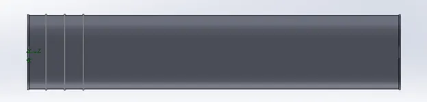
2. The probe lines are made in the cylinder where we need to analyze the flow parameter, velocity with respect to the diametric position. The probe lines are created at 85% (0.15 m from the exit end of the pipe), 90% (0.10 m from the exit end of the pipe) and at 95% (0.5 m from the exit end of the pipe) of the pipe.
   
   The figure below depicts the drawn pipe with the probe lines.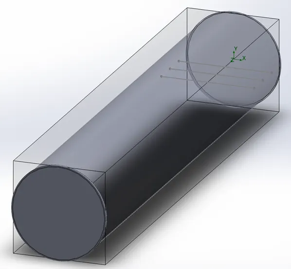
   
   
   
3. For doing the flow analysis, we now move to flow simulation where a new project is created. The parameters such as thermodynamic properties, influence of the gravity, etc. where all set as default and the medium is selected "Water".
   
   
4. The lids are created at the two open region of the pipes so as to provide the boundary conditions at the two pipe ends. Now, it can be visible from the figure that the solidworks have found the domain area by itself where the flow study need to be done.
   
   
   
5. Now boundary conditions are inserted. At the inlet region, the boundary condition given is velocity with a value of `8.9*10^-4 m/s` for the initial case. At the exit region of the static pressure is given as the boundary condition and the wall is selected as real wall, which is again the boundary condition for wall.
   
   
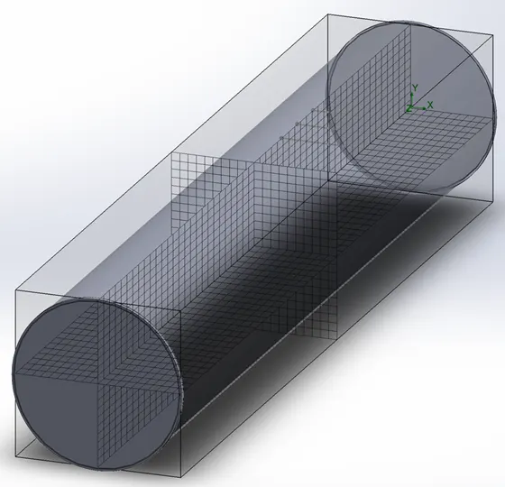
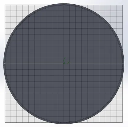
6. The next step is to provide the mesh. This is very important as this is the deciding factor about the accuracy of the solution. More the number of meshes, more will be the accuracy and more will be the time required for solving it. Here, we have inserted 20 meshes along x and y direction, and 54 meshes along z direct which is enough for the chosen dimension of the pipe.
   
   
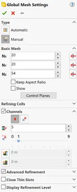
   The obtained meshes are shown below:
   
   
   
   
7. In order to compare the velocities with the diametrical positions at 85%, 90% and 95% positions, a XY plot is created. Each sketch of the line probes at 3 positions are selected and the study parameter chosen is velocity.
8. In order to visualize the flow through pipes, cut planes are created. The cut planes at 85%, 90% and 95% positions are created. A fourth cut plane is created to YZ plane where the complete flow through the pipe can be visualized. For all these cutplanes, the visualizing parameter chosen is velocity.
   
   
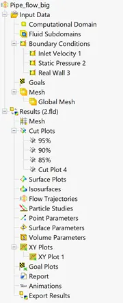
9. Now, the simulation is done the results are obtained.
   
   
10. The parametric study is done in order to find the effect of inlet velocity. The input variable for the parametric study chosen is Velocity normal to the face. The output parameter given is the four cutplanes and the XY plot so as to visualize those cut planes and XY plot for each scenario. Now the scenarios are, the inlet velocity of 0.00089 m/s, 0.0089 m/s and 0.089 m/s for the Reynolds number of 100, 1000 and 10,000. The parametric study is then run.
    
    
    

Output
The following outputs are obtained.

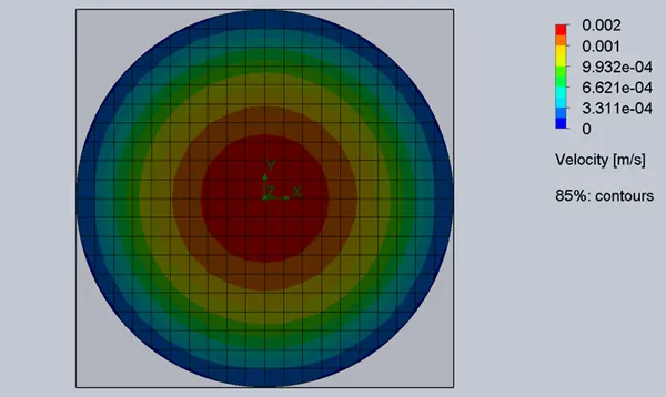
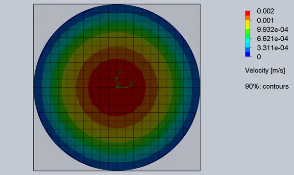
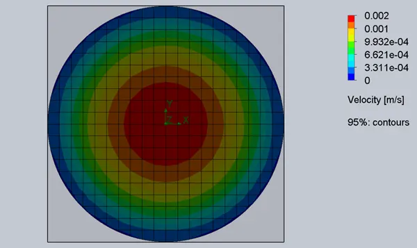
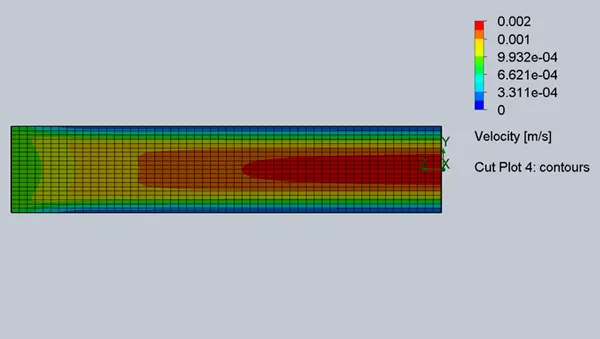
Case 1: Re=100 (v=0.00089 m/s)

1. At probe 85%
   
   
   
2. At probe 90%
   
   
   
3. At probe 95%
   
   
   
4. Cutplane 4
   

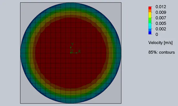
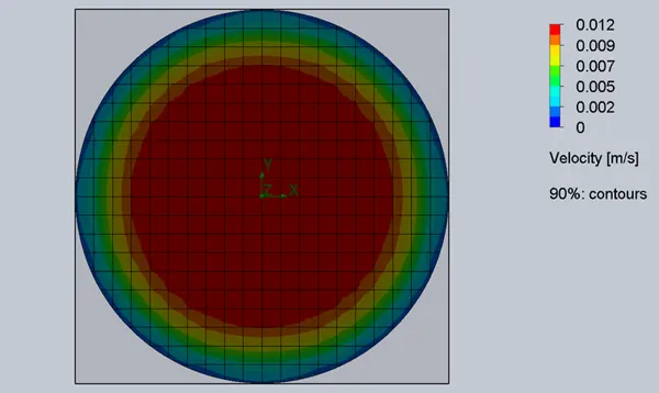
Case 2: Re=1000 (v=0.0089 m/s)

1. At probe 85%
   
   
   
2. At probe 90%
   
   
   
3. At probe 95%
   
   
   
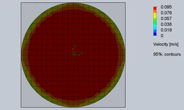
4. Cutplane 4
   

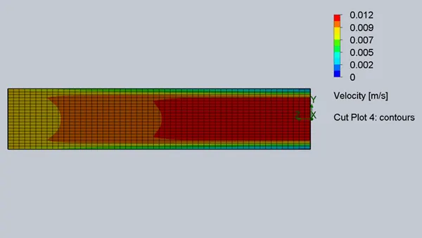
Case 3: Re=10,000 (v=0.089 m/s)

1. At probe 85%
   
   
   
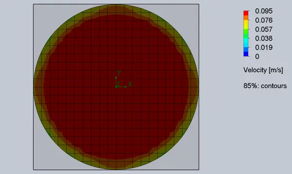
2. At probe 90%
   
   
   
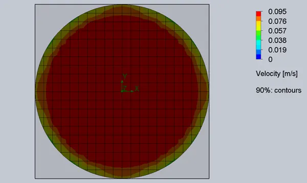
3. At probe 95%
   
   
   
4. Cutplane 4
   

Velocity Comparison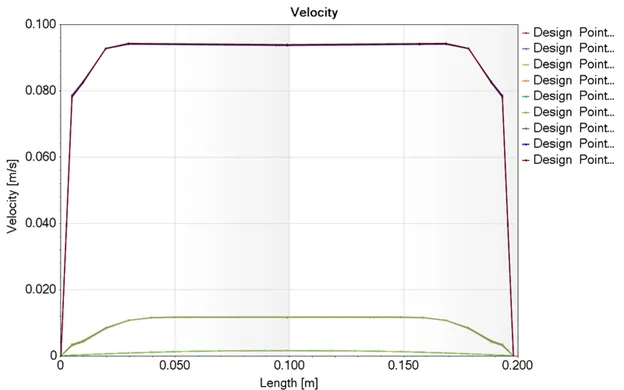


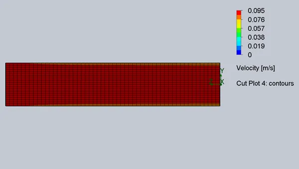
From the above graph, it is clear that the flow pattern changes from laminar to turbulent with increase in the Reynolds Number since the velocity increases. This change of flow pattern to turbulant is visible when compared with the cutplane 4 for each Reynolds number as velocities becomes distorted. The working fluid gets mixed up more when flow changes to turbulent and the effect of viscosity and effect of friction becomes lesser. That is the reason that we can see less of the blue in the cut planes as the velocity increases. Also, no much difference in the velocity is visible between the probe positions at 85%, 90% and 95% for each case of Reynolds number, which is obvious as the probes are very close to each other. Also, the velocity near to the wall decreases with increase in the length of the pipe (cutplane 4 for each case). This is due to the boundary layer formation.

Conclusion
The maximum velocity of fluid through pipe is observed at the center of the pipe. This is due to the fact that the resistance offered is least at the center of the pipe which can be seen using the velocity profile of the fluid flow plotted at the probe, where the parabolic profile can be seen. Due to the formation of the boundary layer, the velocity near the surface is tending to zero.
Increasing the mesh size would increase the accuracy of the result.

Reference

[1] https://www.cati.com/blog/2019/04/introduction-to-computational-fluid-dynamics-with-solidworks-flow-simulation/#:~:text=SOLIDWORKS%20Flow%20Simulation%20enables%20you,create%20products%20with%20superior%20performance.

[2] A Textbook of Fluid Mechanics and Hydraulic Machines, Dr. R.K. Bansal