MATLAB Project: Flow Over Bicycle

Aim
To write a MATLAB Program to calculate the drag force against a cyclist and to plot Velocity and Drag Co-efficient againt Drag Force.

Theory
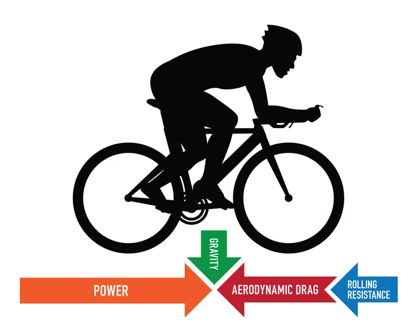
Drag force is the resistance force caused against the motion of a body through a fluid, such as water or air. It acts in the direction opposite to that of the direction of the oncoming flow velocity. In the case of cyclist, he is experiencing a drag force as he is moving against the wind.

(Source: https://www.trainingpeaks.com/blog/understanding-rolling-resistance/)

The magnitude of the drag force on a body depends on the the factors such as Shape of the body, Type of the surrounding fluid and the velocity of the body. The drag co-efficient is the measure of effectiveness of a streamline body shape in reducing the air resistance to the forward motion of the body. The complete area of a body isn't affected rather the projected area is. The projection of a body on the direction of motion is the frontal area. It is this area which experiences drag.

The governing equation to calculate the drag force is,
`F_d = 1/2.C_d. rho.A.v^2`

where, `F_d` is the Drag force [`N`], `A` is the frontal area of the cyclist and bicycle [`m^2`], `rho` is the density of the fluid [`(kg)/m^3`], `C_d` is the coefficient of drag and `v` is the velocity of the cyclist [`m/s`].

Shape Effect on Drag (Variation of drag coefficient with shape) is found in the link: https://www.grc.nasa.gov/WWW/K-12/airplane/shaped.html ----------[1]

Objectives

1. Understanding the concept of Drag force.
2. Construct a MATLAB program to calculate drag force.
3. Plot the graph Velocity vs Drag force and study the variation and responsible variables.
4. Plot the graph Drag Coefficent vs Drag force and study its variation.

Program to plot Velocity vs Drag Force
Here, the cyclist is assumed to be flat plane. Therefore, the drag coefficient, C_d=1.28 (from [1]). The density of the fluid is air, rho=1.225 kg/m^3. The frontal area which is responsible for drag is as assumed to be 1.2m^2.

For the studying the variation of Draf force with respect to velocity, we can assume that the cylist can travel upto 15m/s (ie, 54 km/hr). Therefore, velocity varies from 0 to 15 m/s.

% Challenge: Flow over bicycle;
% Plot Velocity vs Drag Force;
clear all
close all
clc

% Assigning values to the known factors.
C_d = 1.28;
rho = 1.223;
A = 1.2;

% v= 0 to 15 is assigned using linspace command and 30 divisions assigned
% for the graph to have smooth lines.
v = linspace(0,15,30);

% Calculation of F_d for each value of v.
F_d = 0.5*C_d*rho*A*v.^2;

% Plotting
%color and marking for the curve is given using keyword 'color'&'marker'
%x-axis and y-axis is labeled usin keywords xlabel and ylabel
%grid on is used to make the grid appear on graph
%grid minor is used to increase the no.of grid lines 
plot(v,F_d,'color','r','marker','*');
xlabel('Velocity, m/s');
ylabel('Drag Force, N');
grid on;
grid minor;

Output of the Program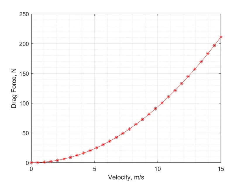

As from the equation, drag force (`F_d`) is propotional to the square of velocity, which is implied through the graph. That is, if velocity is increased twice, then the drag force increment will be 4 times which is not good as the drag force is basically the air resistance pushing in the opposite side of the direction of motion of the cyclist.

Program to plot Velocity vs Drag Force (for different frontal area in a single graph)
In the above program, the frontal area was assumed to be flat plane. Now, let's study the variation of drag force w.r.t velocity for different frontal areas.

From [1], the coefficent of drag for different frontal areas were found. This include Flat Plate, Prism, Bullet, Sphere and Aerofoil. According to [1],
Drag coefficient of Flat Plate, C_d_f=1.28
Drag coefficient of Prism, C_d_p=1.14
Drag coefficient of Bullet, C_d_b=0.295
Drag coefficient of Sphere, C_d_s=0.07 to 0.5
Drag coefficient of Aerofoil, C_d_a=0.045

% Challenge: Flow over bicycle;
% Plot Velocity vs Drag Force for different frontal shapes of same frontal
% area.
clear all
close all
clc

% Assigning values to the known factors.
C_d_f = 1.28;
C_d_p = 1.14;
C_d_b = 0.295;
C_d_s = 0.260;   %average value for sphere
C_d_a = 0.045;
rho = 1.223;
A = 1.2;

% v= 0 to 15 is assigned using linspace command and 30 divisions assigned
% for the graph to have smooth lines.
v = linspace(0,15,30);

% Calculation of F_d for each value of v (for different drag coefficeints).
F_d_f = 0.5*C_d_f*rho*A*v.^2;
F_d_p = 0.5*C_d_p*rho*A*v.^2;
F_d_b = 0.5*C_d_b*rho*A*v.^2;
F_d_s = 0.5*C_d_s*rho*A*v.^2;
F_d_a = 0.5*C_d_a*rho*A*v.^2;

% Plotting
%hold on and hold off are used to make the different curve appear on same graph
%different color is given for each frontal shape using keyword 'color'
%legend keyword is used to label each curve in the graph
%x-axis and y-axis is labeled usin keywords xlabel and ylabel
%grid on is used to make the grid appear on graph
hold on;
plot(v,F_d_f,'color','r','marker','*');
plot(v,F_d_p,'color','g','marker','*');
plot(v,F_d_b,'color','m','marker','*');
plot(v,F_d_s,'color','b','marker','*');
plot(v,F_d_a,'color','k','marker','*');
legend('Flat Plane','Prism','Bullet','Sphere','Aerofoil');
hold off;
xlabel('Velocity, m/s');
ylabel('Drag Force, N');
grid on;
grid minor;

Output of the Program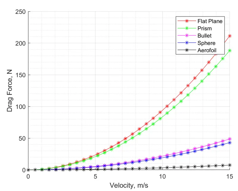

As the frontal shape changes (for same frontal area), the drag coefficient also changes. The less the drag coefficient is, the lesser will be the drag force, and less will be the air resistance against the direction of the cyclist. So from the graph, the drag force is less seen for aerofoil shape, followed by sphere, bullet, prism and flat plane which concludes that the aerofoil shape should be preferred over other shapes inorder to minimise the drag force.

Program to plot Drag Co-efficent vs Drag Force
From [1], the coefficent of drag for different frontal areas were found. This include Flat Plate, Prism, Bullet, Sphere and Aerofoil. According to [1],
Drag coefficient of Flat Plate, C_d_f=1.28
Drag coefficient of Prism, C_d_p=1.14
Drag coefficient of Bullet, C_d_b=0.295
Drag coefficient of Sphere, C_d_s=0.07 to 0.5
Drag coefficient of Aerofoil, C_d_a=0.045

% Challenge: Flow over bicycle;
% Plot Drag co-efficient vs Drag Force;
clear all
close all
clc

% Assigning values to the known factors.
C_d = [0,0.045,0.260,0.295,1.14,1.28]; %for different shapes
rho = 1.223; 
A = 1.2; %assumption
v = 15; %assumptiom

% Calculation of F_d for each value of C_d.
F_d = 0.5.*C_d*rho*A*v^2;

% Plotting
%x-axis and y-axis is labeled usin keywords xlabel and ylabel
%grid on is used to make the grid appear on graph
%grid minor is used to increase the no.of grid lines 
%text command is used to plot specific points on the curve;
plot(C_d,F_d,'color','r','marker','*');
xlabel('Drag Co-efficient');
ylabel('Drag Force, N');
text(C_d(2),F_d(2),'Aerofoil');
text(C_d(3),F_d(3),'Sphere');
text(C_d(4),F_d(4),'Bullet');
text(C_d(5),F_d(5),'Prism');
text(C_d(6),F_d(6),'Flat Plate');
grid on;
grid minor;

Output of the Program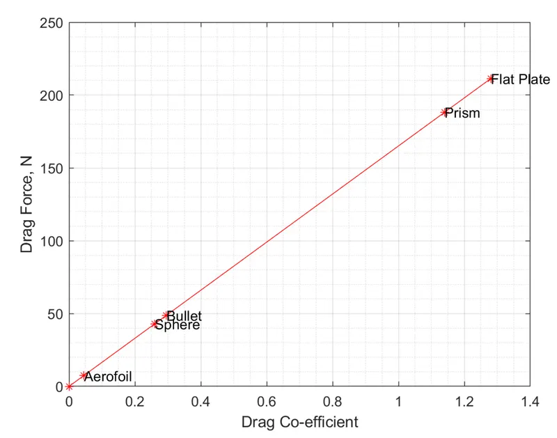

The curve obtained in Drag force vs drag co-efficient is a straight line which is obvious as drag force directly proportional to drag co-efficient. The drag co-efficient is depended on the shape irrespective frontal area, ie, the drag co-efficient is different for different shapes even though their frontal area is same.

From the figure, it shows that the drag force is minimum for aerofoil shape followed by sphere, bullet, prism and flat plate. So in order to reduce the drag force, the shape should be opted corresponding to the lower drag co-efficient. That is, shape does an important role in producing drag force.

Conclusion
The MATLAB program to compute the Drag Force has been successfully created. The Velocity vs Drag Force graph and the Drag Co-efficent vs Drag Force graphs has been successfully created using the program and the variation of the graph has been studied.