MATLAB Project: Air Standard Cycle

Aim
To create a MATLAB Program to solve an OTTO Cycle and make its plots. Also to calculate the thermal efficiency of the Engine.

Theory
The Otto Cycle is an idealized thermodynamic cycle consisting of a set of processes used by Spark Ignition (SI) internal combustion engines. It describes how heat engines turn gasoline into motion. These engines would ingest a mixture of fuel and air, compress it and cause it to react, thus effectively adding heat through converting chemical energy into thermal energy. These expanded combustion products are ejected and replaced them with new charge of fuel and air. The Otto Cycle provides the energy for most transportation and was essential for the modern world [1].

The PV diagram of the ideal Otto cycle is shown in figure 1. It explains how the changes in pressure and volume of the working fluid (gasoline and air mixture) change due to combustion which powers the movements of a piston, creating heat, to provide motion of vehicle [2]. 

Figure 1: The ideal Otto Cycle [3].

The different process in the Figure 1 are [4]:
Process 5 → 1: mass of air is drawn into piston/cylinder arrangement at constant pressure.
Process 1 → 2: adiabatic (isentropic) compression of the charge as the piston moves from bottom dead center (BDC) to top dead center (TDC). 
Process 2 → 3: constant volume heat transfer to the working gas from an external source while piston is at top dead center. This process is intended to represent the ignition of the air-fuel mixture and the subsequent  rapid burning.
Process 3 → 4: adiabatic (isentropic) expansion (power stroke).
Process 4 → 1: constant volume process in which heat is rejected from the air while the piston is at the bottom dead center.
Process 1 → 5: mass of air is released to the atmosphere in a constant pressure process.

The actual cycle does not have the sharp transitions between the different processes and the ideal cycle might be as sketched in Figure 2.

Figure 2: Sketch of an actual Otto cycle [2]. 

Efficiency of an Ideal Otto Cycle
It is defined as the ratio between work done during Otto cycle to the heat supplied during Otto cycle.

 
 
 

Process 1 → 2 is an isentropic (reversible adiabatic) process. For this process, the relation between T and V is as follows:
   

Similarly, Process 3 → 4 is also an isentropic process. Therefore,

Subtituting (ii) and (iii) in (i). We get thermal efficiency as,
  
is the equation for Thermal efficiency of an Otto Cycle.

Relation between Crank Angle and Volume inside Crank Chamber
  
where, V is the volume inside crank chamber, `V_c` is the clearance volume, `r_c` is the compression ratio and R is the ratio of length of connecting rod to crank pin radius.

Engine Parameters
Bore = 0.1m
Stroke = 0.1m
Length of connecting rod, con_rod = 0.15m
Compression ratio, cr = 12
Crank pin radius, a = Stroke/2 [unit:m]

Program

% OTTO Cycle

clear all
close all
clc

% Engine Parameters
bore = 0.1;
stroke = 0.1;
con_rod = 0.15; %connectin rod length
cr = 12; %compression ratio
a = stroke/2; %crank pin radius
R = con_rod/a;

% Specific heat ratio
gamma = 1.4;

�lculating the swept colume and clearance volume
v_swept = (pi/4)*(bore^2)*stroke;
v_clearance = v_swept/(cr-1);

v1 = v_swept+v_clearance;
v2 = v_clearance;

% State Variables at point 1
p1 = 101325;   
t1 = 500;       %assumption, in Kelvin

% State Variables at point 2
p2 = p1*(cr^gamma);
t2 = p2*v2*t1/(p1*v1);  %Ideal gas equation
% Explanation: process 1->2, isentropic process
%               p1.v1^gamma = p2.v2^gamma; cr=v1/v2

% Process 1 to 2, Isentropic compression
v_compression = volume_calculation(cr,R,v_clearance,180,0);
c_12 = p1*(v1^gamma);
p_compression = c_12./(v_compression).^gamma;

% State Variables at point 3
v3 = v2;
t3 = 2300; %assuming maximum temp of combustion process as 2300K
p3 = p2*(t3/t2); %Ideal gas equation (v2=v3)

% State Variables at point 4
v4 = v1;
p4 = p3*(v3/v4)^gamma;
% Explanation: process 3->4, isentropic process
%               p3.v3^gamma = p4.v4^gamma;

% Process 3 to 4, Isentropic expansion
v_expansion = volume_calculation(cr,R,v_clearance,0,180);
c_34 = p3*(v3^gamma);
p_expansion = c_34./(v_expansion).^gamma;

hold on;

plot(v_compression,p_compression,'color','b','linewidth',1.2);
plot([v2 v3],[p2 p3],'color','m','linewidth',1.2);
plot(v_expansion,p_expansion,'color','g','linewidth',1.2);
plot([v4 v1],[p4 p1],'color','r','linewidth',1.2);
legend('Process 1 to 2: Isentropic Compression','Process 2 to 3: Constant volume heat addition','Process 3 to 4: Isentropic Expansion','Process 4 to 1: Constant volume heat rejection');

text(v1,p1-0.05e6,'1');
text(v2,p2,'2');
text(v3,p3,'3');
text(v4,p4+0.08e6,'4');
xlabel('Volume, m^3');
ylabel('Pressure, Pa');
title('PV diagram of an Otto Cycle');

�lculation of Thermal efficiency
eff = 1-(1/(cr^(gamma-1)));
fprintf('Thermal Efficiency is %2.4f%% n',eff*100); %to print thermal efficiency

Each step of the function is explained with comments.

Further explanation:
For isentropic processes (Process 1 to 2 and process 3 to 4), the volume for each process is calculated by a function, 'volume_calculation' with inputs as cr, R, v_clearance, start_theta and end_theta. The start_theta and end_theta are basically the initial and final value of the angle possessed by the crank shaft for those isentropic process. For compression, the value ranges from 180 to 360 degree while for expansion process it varies from 0 to 180.

The function volume_calculation with it's input argument return the value found to the varaible (here, v_compression and v_expansion) when it is called. The function volume_calculation is defined below:

function [V] = volume_calculation(cr,R,v_clearance,start_theta,end_theta)


% Volume Calculation

theta = linspace(start_theta,end_theta,180);

V = (1+(0.5*(cr-1)*(R+1-cosd(theta)-(R^2-(sind(theta)).^2).^0.5)))*v_clearance;

The text command in the main code has alloted the exact co-ordinate value for points 2 and 3. But the co-ordinate points for points 1 and 4 has been sligthly moved up and down from it's actual value so as to make sure that the points 1 and 4 marked on the plot using the text command does not collide or touch each other, so that each point will be properly visible on the graph. This happened since the points 1 and 4 are very close to each other.

Result
The MATLAB program to plot the PV diagram of an Otto cycle has been coded successfully and it's required graph has been obtained.

The obtained PV diagram is,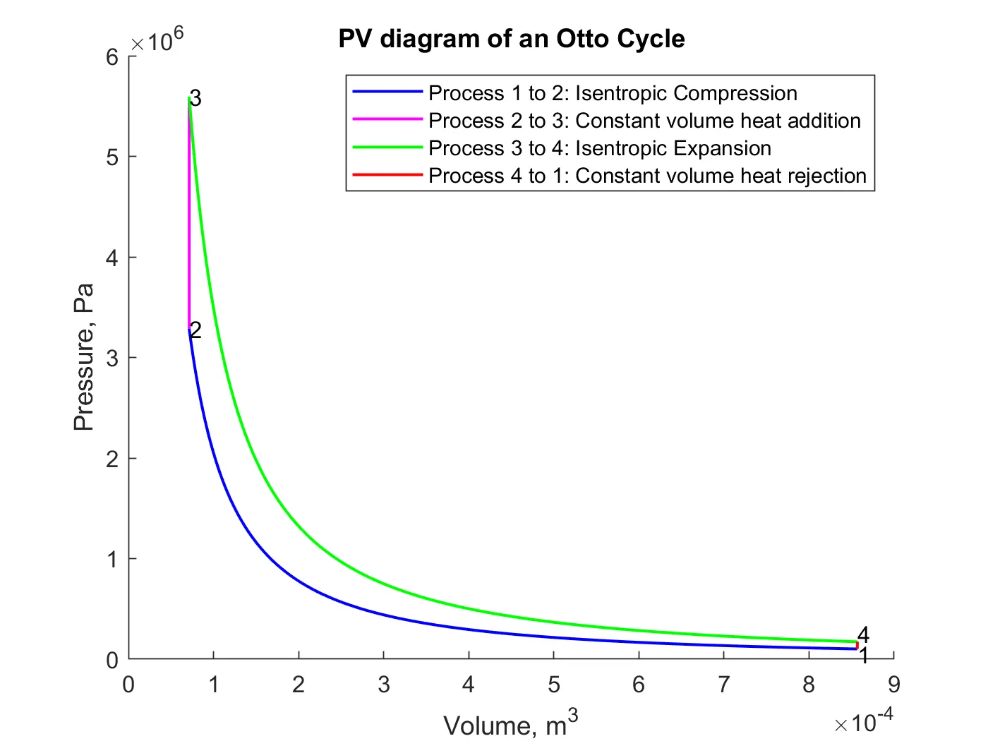

The Thermal efficieny of the Otto cycle has been found as 62.9893%.

The screenshot of the command window showing the thermal efficiency is shown below: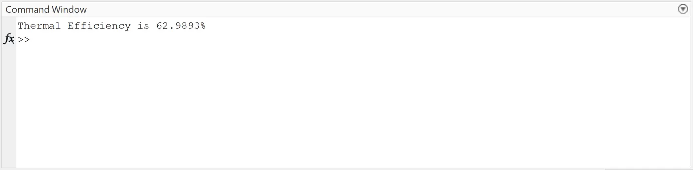

References
[1] https://www.grc.nasa.gov/WWW/K-12/airplane/otto.html
[2] https://energyeducation.ca/encyclopedia/Otto_cycle
[3] https://web.mit.edu/16.unified/www/FALL/thermodynamics/notes/node26.html
[4] https://en.wikipedia.org/wiki/Otto_cycle
[5] https://www.sciencedirect.com/topics/engineering/otto-cycle