MATLAB Project: Solving second order ODEs
Aim:
To write a MATLAB program to solve the second order differential equation and to simulate the pendulum motion.
Theory:
A differential equation is an equation with a function and one or more of its derivatives [1].
`y+dy/dx=5x`: It is a differential equation with the function `y` and its derivative `dy/dx`.
The Order of the differential equation is the highest derivative.
A simple representation of Second order differential equation is,
`(d^2y)/(dx^2) +P(x)*dy/dx+Q(x)*y = f(x)`
where, `P(x)`, `Q(x)`and `f(x)`are functions of x.
For the function to be homogeneous, `f(x)`=0.
ie, `(d^2y)/(dx^2)+P(x)*dy/dx+Q(x)*y=0`
Also, if the functions `P(x)`and `Q(x)` are constants `p` and `q`, then,
`(d^2y)/(dx^2)+p*dy/dx+q*y=0`
In engineering, ODE is used to describe the transient behaviour of a system. An example is a simple pendulum.
The Equation of Motion of a Simple Pendulum
A pendulum is body suspended from a fixed support so that it swings freely back and forth under the influence of gravity [2]. So when a pendulum is displaced sideways from its resting or the equilibrium position, it is subject to a restoring force due to gravity that will accelerate it back towards the equilibrium position. So the pendulum will swing back and forth with periodic motion, if it displaced to an initial angle and released [3].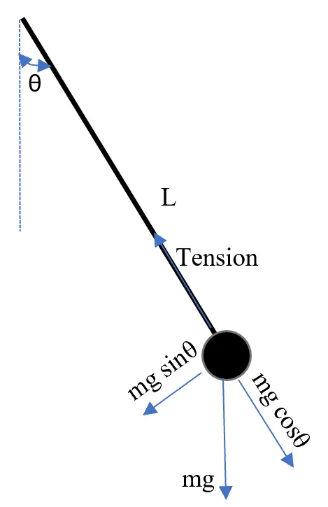
Figure 1: Representation of Simple Pendulum
The simple pendulum consists of a mass `m` hanged from a straight string of length `L` and fixed at a pivot point. The way the pendulum moves depends on the Newton's second law.The differential equation which represents the motion of a simple pendulum is,
`(d^2theta)/dt^2 = b/m*( dtheta)/dt + g/l*sintheta = 0`...............(Equation 1)
where, `g` is the acceleration due to gravity, `b` is the damping coefficient, `l` is the length of the pendulum and `theta` is the angular displacement
This system is equivalent to the mass attached to spring and damper system. Is has various applications such as, in vehicle dynamics, suspension system can be modelled as a set of mass, spring and damper using the equation of motion of this system. This reveals the significance of the solution to this equation.
Generally, the higher order ODEs are solved by breaking it into first order ODEs. For solving the second order ODE, same approach can be used in MATLAB by makin use of the ode45 command.
For solving Equation 1,
Let `theta_2 = (dtheta_1)/dt`..................(Equation 2)
when Equation 2 is equated with Equation 1, we get,
`(dtheta_2)/dt=-b/m*theta_2-g/l*sintheta_1`
ie, `d/dt [[theta_1],[theta_2]]=[[theta_2],[-b/mtheta_2-g/lsintheta_1]]`
where the matrix on the LHS is the solution vector because it is this values we are finding out using the ode45 function.
Objectives:
- Understanding the theoretical concept of Simple pendulum and the solving of the Ordinary differential equation.
- Understanding the ode45 command in MATLAB that to be used for solving the ODE in the MATLAB program.
- Writing a program in MATLAB to solve the equation of motion of simple pendulum (second order ODE) and to plot the angular displacement and angular velocity graph with respect to time.
- Modifying the program to simulate the pendulum motion and to create a movie of it.
Program to solve ODE :
The programming is done in MATLAB.
% Solving 2nd order Ordinary differential equation
clear all
close all
clc

% Parameters
b = 0.05;
g = 9.81; % m/s^2
l = 1; % m
m = 1; % kg

% Initial Condition
i_c = [0;3];  %assigning angular displacement=0, angular velocity=3 rad/sec

% Time Points
t_span = linspace(0,20,1000);  % motion from 0 to 20 seconds

% Solve ODE
[t, result] = ode45(@(t,theta) ode_func(t,theta,b,g,l,m),t_span,i_c);
%result value will be consisting of 2 columns, where first column will be
%values of displacement and the other will be velocity

% Plotting Dispacement and velocity w.r.t. time

    subplot(2,1,1);
    plot(t,result(:,1));
    xlabel('Time, s');
    ylabel('Angular Displacement, rad');
    axis([0 20 -1.5 1.5]);
    hold on;
    grid on;
    grid minor;
    title('Angular displacement vs time');

    subplot(2,1,2);
    plot(t,result(:,2));
    xlabel('Time, s');
    ylabel(' Angular Velocity, rad/s');
    axis([0 20 -5 5]);
    grid on;
    grid minor;
    title('Angular velocity vs time');
Each step of the program is explained with comments.
Function definiton of the function ode_func is given below:
function [dtheta_dt] = ode_func(t,theta,b,g,l,m)

dtheta1_dt = theta(2);
dtheta2_dt = (-(b/m)*theta(2))-((g/l)*sin(theta(1)));
dtheta_dt = [dtheta1_dt; dtheta2_dt];
end
The function ode_func takes the value b, g, l and m as input parameters. This ode_func has two inputs, t and theta, apart from the other arguments., where t would be the current time and theta would be the value of function at the previous time step.
Output of the program: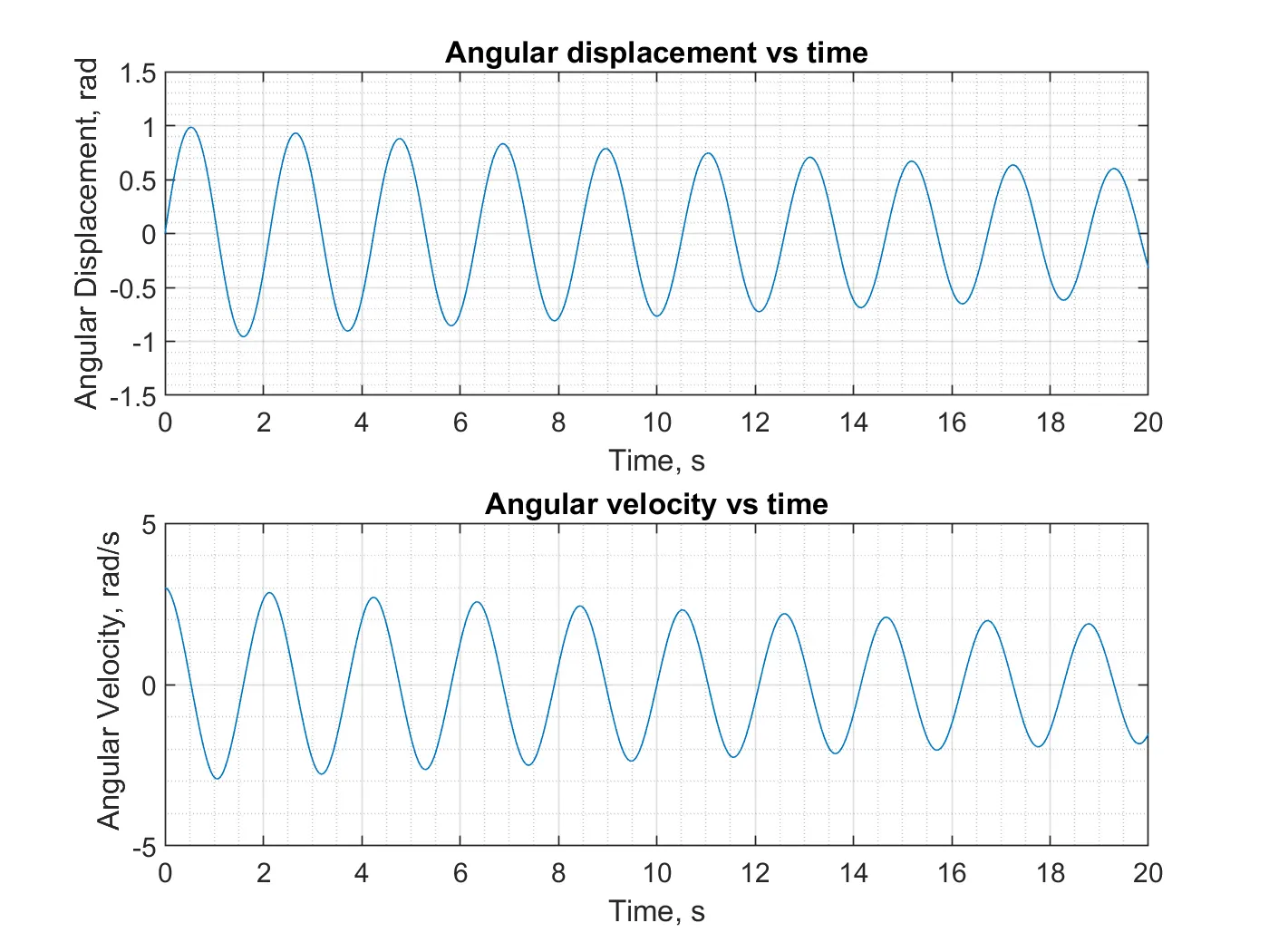
The plot/graph obtained for the corresponding program is shown above.
ode45 command
ode45 is function in MATLAB that solves ordinary or partial differential equations using the numerical method, Runge Kutta method, which is a first order ODE solver for initial value problems. Here, we are providing intial condition, angular displacement as 0 and angular velocity as 3 rad/s using the variable i_c. The ode45 function would use the 4th order RK method to solve for the solution.
The function ode45 takes 3 inputs, which are
- Function to be integrated. Here, ode_func is the function to be integrated and this funtion should contains at least 2 inputs (here, t and theta) apart from the other arguments. t would be the current time and theta would be the value of the function at the previous time step.
- Time span. The time span would be the integration limits. Here, t_span variable is used where its lower and upper limit are specified using the linspace function. The solver will choose a step size that is most suitable for the solution to obtain the solution in the most optimal time as possible.
- Initial conditions. The initial condition would be the value of the function at t=0. Here, initial condition is provide using the variable i_c where the angular displacement and angular velocity are provided (here, 0 and 3).
Since the RK method is a first order ODE solver and hence, so is ode45. Thus, ODE to be integrated by ode45 must be provided as a set of first order ODEs. (Refer theory section to know how the equation of motion of simple pendulum, which is 2nd order ODE is converted into a set of 2 first order ODE by using the variable `theta_2`.
Program to simulate the pendulum motion:
The programming is done in MATLAB.
% Solving 2nd order Ordinary differential equation
clear all
close all
clc

% Parameters
b = 0.05;
g = 9.81;
l = 1;
m = 1;

% Initial Condition
i_c = [0;3];

% Time Points
t_span = linspace(0,20,1000);

% Solve ODE
[t, result] = ode45(@(t,theta) ode_func(t,theta,b,g,l,m),t_span,i_c);
%result value will be consisting of 2 columns, where first column will be
%values of displacement and the other will be velocity

% Plotting Dispacement and velocity w.r.t. time

    subplot(6,5,[21,22,26,27]);
    plot(t,result(:,1));
    xlabel('Time, s');
    ylabel('Angular Displacement, rad');
    axis([0 11 -1.5 1.5]);
    hold on;
    grid on;
    grid minor;

    subplot(6,5,[24,25,29,30]);
    plot(t,result(:,2));
    xlabel('Time, s');
    ylabel(' Angular Velocity, rad/s');
    axis([0 11 -5 5]);
    grid on;
    grid minor;

    % f_no is the frame number; Initialising its value as 1
    f_no = 1;

for i = 1:length(result(:,1))
    x1 = l.*sin(result(i,1));
    y1 = -l.*cos(result(i,1));

    subplot(6,5,[21,22,26,27]);
    plot(t(i),result(i,1),'marker','.','color','r','linewidth',0.5);
    axis([0 20 -1.5 1.5]);

    subplot(6,5,[24,25,29,30]);
    hold on;
    plot(t(i),result(i,2),'marker','.','color','r','linewidth',0.5);
    hold off;
    axis([0 20 -5 5]);

    subplot(6,5,[1:15]);
    plot([0 x1],[0 y1],'color','m','linewidth',1.3);
    hold on;
    line([-0.5 0.5],[0 0],'linewidth',3,'color','k');
    plot(x1,y1,'marker','o','color','b','linewidth',7);
    format short;
    disp_t = t(i);
    txt = ['Time = ' num2str(disp_t) ' s'];
    text(0.70,0,txt);
    title('Simple Pendulum');
    hold off;
    axis([-1.7 1.7 -1.25 0.15]);
    pause(0.001);

    % Recording Frames;
        M(f_no) = getframe(gcf); %capture each position to the variable M;
        f_no = f_no+1;           %increment of frame no.

end

% Making Movie
movie(M);  %plays movie of the frames captured in M
videofile = VideoWriter('simple_pendulum.avi','Uncompressed AVI'); %write video data as AVI file into videofile
open(videofile) %open video file
writeVideo(videofile,M) %to create a video file from the array "M"
close(videofile) %close video file
The function definition of ode_func is given below:
function [dtheta_dt] = ode_func(t,theta,b,g,l,m)

dtheta1_dt = theta(2);
dtheta2_dt = (-(b/m)*theta(2))-((g/l)*sin(theta(1)));
dtheta_dt = [dtheta1_dt; dtheta2_dt];
end
For creating an animation, a for loop is generated.
The variable result will have two columns after solving the differential equation using ode45. The first column represents the displacement angle for each value of time t. Similarly, the second column of the variable result contains the angular velocity for each value of t. In order to represent the displacement and angular velocity w.r.t time and the animation of pendulum in a single plot, the command 'subplot' has been used. The position to represent each subplot ideally has been found by trying with various inputs (trial and error method).
The two subplots can be seen outside the for loop. That is done in order to have the curve on the displacement and velocity w.r.t time graphs. These same subplots present in the for loop indicates the corresponding values using the red points. This can be understood properly when viewing the result video.
For animating the simple pendulum, the plot has been created joining the two points, fixed points (0,0) and the corresponding points of angular displacement from the variable result (column 1) by trigonometric calculation. For representing the ball of the pendulum, again the point corresponding to the angular displacement has been plotted and the 'o' marker is used.
For indicating the current time in the simple pendulum animation, the text command is used to indicate the required text at a particular point on the plot. For creating a movie, the variable f_no has been used to indicate the frame number. The variable M is allocated each frame of the plot and the new video file named 'simple_pendulum' in AVI format is been created.
Output of the Program:
The video out of the corresponding MATLAB program is shown below:
video link: https://youtu.be/UDxjrWVozMg
Conclusion:
The MATLAB program to solve the second order ODE has been successfully created.
The governing equation of the simple pendulum has been solved and graphs showing the variation of position and angular velocity with time has been plotted.
The ode45 function has been used to solve the ODE and the pendulum motion has been simulated. From the graphs and animation, it shows that the pendulum motion is more and continuous due to the low damping coefficient. Increasing te damping coefficient would increases the resistance to flow.
Errors faced while programming:
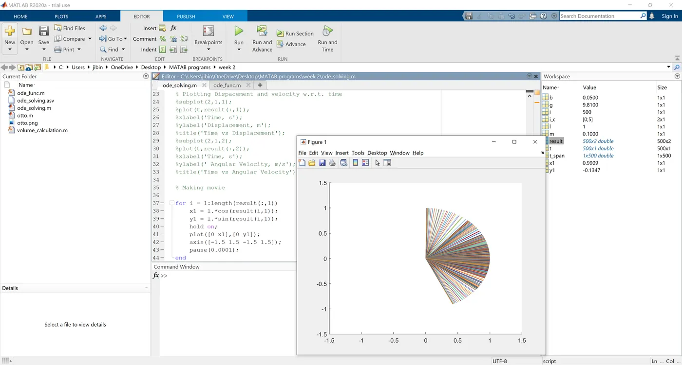
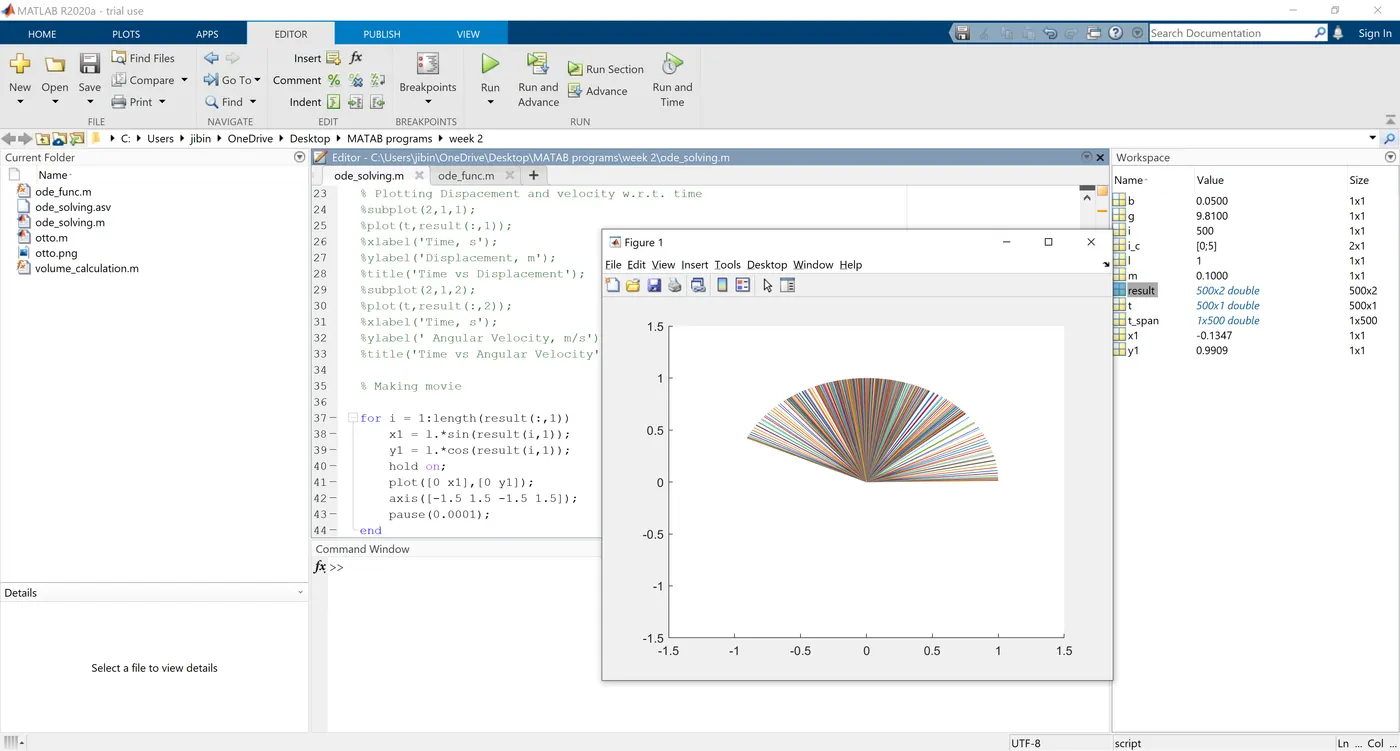
- The orientation of the pendulum was wrong. This was corrected by introducing -ve sign to the cos function and properly giving trigonometric function to variables x1 and y1.
References:
[1] https://www.mathsisfun.com/calculus/differential-equations-second-order.html#:~:text=where%20P(x)%2C%20Q,a%20wider%20range%20of%20functions.
[2] https://en.wikipedia.org/wiki/Pendulum_(mathematics)
[3] https://www.acs.psu.edu/drussell/Demos/Pendulum/Pendula.html
[4] https://www.acs.psu.edu/drussell/Demos/Pendulum/Pendulum.html#:~:text=By%20applying%20Newton's%20secont%20law,enough%2C%20so%20the%20small%20angle
[5] http://hyperphysics.phy-astr.gsu.edu/hbase/pend.html
[6] https://www.khanacademy.org/science/ap-physics-1/simple-harmonic-motion-ap/simple-pendulums-ap/a/simple-pendulum-ap1
[7] https://in.mathworks.com/help/matlab/ref/subplot.html