PYTHON Project: Drag Force of a Cyclist
Aim
To write a PYTHON program to calculate the drag force against a cyclist and to plot Velocity and Drag Co-efficient against Drag Force.
Theory
Drag force is the resistance force caused against the motion of the body through a fluid, such as water or air. It acts in the direction opposite to that of the direction of the oncoming flow velocity. In the case of the cyclist, he is experiencing a dra force as he is moving against the wind.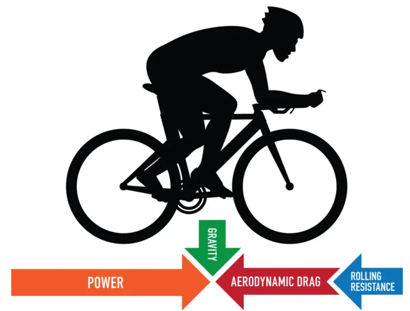
Figure 1: Motion of the cyclist and aerodynamic drag [1].
The magnitude of the drag force on a body depends on the factors such as shape of the body, type of the surrounding fluid and the velocity of the body. The drag co-efficient is the measure of effectiveness of a streamline body shape in reducing the air resistance to the forward motion of the body. The complete area of a body isn't affected rather the projected area is. It is the area which experiences drag.
The governing equation to calculate the drag force is,
`F_d = 1/2.C_d.rho.A.v^2`
where, `F_d` is the Drag Force `[N]`, `A` is the frontal area of the cyclist and bicycle `[M^2]`, `rho` is the density of the fluid `(kg)/m^3`, `C_d` is the coefficient of drag and `v` is the velocity of the cyclist `[m/s]`.
Shape effect on drag (variation of drag coefficient with shape) is found in the link:
https://www.grc.nasa.gov/WWW/K-12/airplane/shaped.html
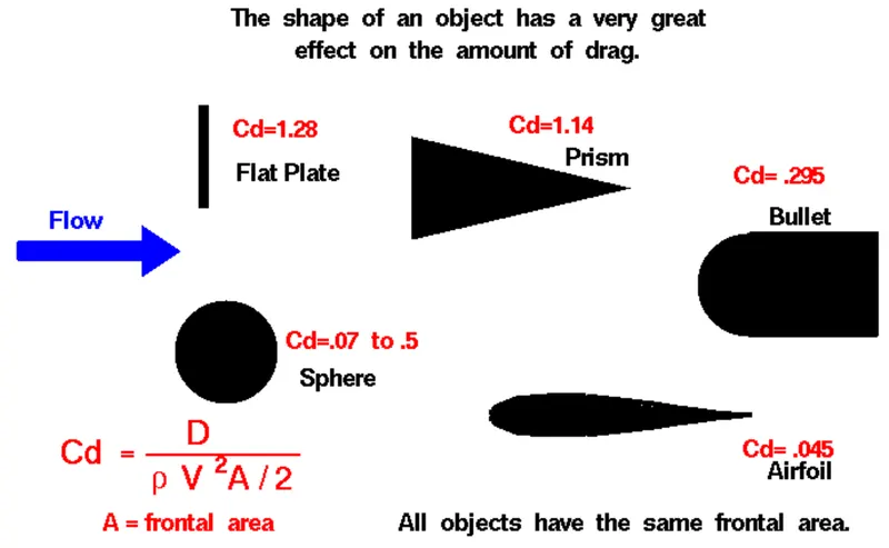
Figure 2: Drag coefficient for various shapes for same frontal area [2].
Objectives
- Understanding the concept of Drag force.
- Construct a PYTHON program to calculate drag force.
- Plot the graph Velocity vs Drag force, and study the variation and responsible variables.
- Plot the graph Drag Coefficient vs Drag Force, and study its variation.
Program to plot Velocity vs Drag Force
Here, the cyclist is assumed to be a flat plate. Therefore, the drag coefficient `C_d` of 1.28 is assumed (from [2]). The density of fluid (air) is taken as, `rho`= 1.225 `(kg)/m^3`. The frontal area which is responsible for the drag is assumed to be 1.2 `m^2`.
For studing the variation of Drag force with respect to velocity, it is assumed that the cyclist can travel upto 15`m/s` (ie., 54 `(km)/(hr)`). Therefore, the velocity varies from 0 to 15 `m/s`.
# Flow Over a Bicycle
# Plot Velocity vs Drag Force

import math
import matplotlib.pyplot as plt
import numpy as np

# Assigning values to the known factors
C_d = 1.28
rho = 1.223
A = 1.2

# assigning velocity values from 0 to 15 using linspace command
v = np.linspace(0,15,30)  #30 divisions

# calculation of drag force
F_d = 0.5*C_d*rho*A*np.array(v)*np.array(v)

# PLOTTING
plt.plot(v,F_d,'k',v,F_d,'r*')
plt.xlabel('Velocity, m/s')
plt.ylabel('Drag Force, N')
plt.title('Velocity vs Drag Force')
plt.show()
Output of the Program
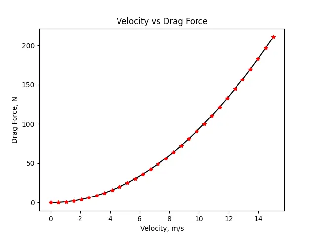
From the equation, drag force (`F_d`) is proportional to the square of velocity, which is implied through the graph. That is, if the velocity is increased twice, then the drag force increment will be four times which is not good, as the drag force is basically the air resistance acting opposite side of movement of the cyclist.
Program to plot Velocity vs Drag Force (for different frontal area in a single graph)
In the above program, the frontal area was assumed to be a flat plate. Now, the study is done variation of drag force with respect to velocity for different frontal areas.
From [2], the coefficient of drag for different frontal areas were found. This include flat plate, prism, bullet, sphere, and aerofoil. According to [2],
Drag coefficient of Flat plat, C_d_f = 1.28
Drag coefficient of Prism, C_d_p = 1.14
Drag coefficient of Bullet, C_d_b = 0.295
Drag coefficient of Sphere, C_d_s = 0.07 to 0.5
Drag coefficient of Aerofoil, C_d_a = 0.045
# Flow Over a Bicycle

# Plot Velocity vs Drag Force for different frontal shapes

import math
import matplotlib.pyplot as plt
import numpy as np

# Assigning values to the known factors
C_d_f = 1.28	# flat plane
C_d_p = 1.14	# prism
C_d_b = 0.295	# bullet
C_d_s = 0.260	# sphere
C_d_a = 0.045	# aerofoil
rho = 1.223
A = 1.2

# assigning velocity values from 0 to 15 using linspace command
v = np.linspace(0,15,30)  #30 divisions

# calculation of drag force
F_d_f = 0.5*C_d_f*rho*A*np.array(v)*np.array(v)
F_d_p = 0.5*C_d_p*rho*A*np.array(v)*np.array(v)
F_d_b = 0.5*C_d_b*rho*A*np.array(v)*np.array(v)
F_d_s = 0.5*C_d_s*rho*A*np.array(v)*np.array(v)
F_d_a = 0.5*C_d_a*rho*A*np.array(v)*np.array(v)


# PLOTTING
plt.plot(v,F_d_f,'r', label="Flat Plane")
plt.plot(v,F_d_p,'k', label="Prism")
plt.plot(v,F_d_b,'m', label="Bullet")
plt.plot(v,F_d_s,'g', label="Sphere")
plt.plot(v,F_d_a,'b', label="Aerofoil")
plt.legend(loc="upper left") 	# defining position for legend
plt.xlabel('Velocity, m/s')
plt.ylabel('Drag Force, N')
plt.title('Velocity vs Drag Force')
plt.show()
Output of the Program
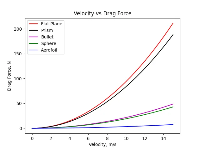
As the frontal shape changes (for same frontal area), the drag coefficient also changes. The less the drag is , the lesser will be the drag force, and less will be the air resistance against the direction of the cyclist. From the graph, the drag force is seen less for aerofoil shape, followed by sphere, bullet, prism and flat plate which concludes that the aerofoil shape should be preferred over other shapes in order to minimise drag force.
Program to plot Drag Co-efficient vs Drag Force
From [2], the coefficent of drag for different frontal areas were found for different shapes such as Flat Plate (1.28), Prism (1.14), Bullet (0.295), Sphere (0.07 to 0.5), and Aerofoil (0.045).
# Flow Over a Bicycle

# Plot Drag Coefficient vs Drag Force for different frontal shapes

import math
import matplotlib.pyplot as plt
import numpy as np

# Assigning values to the known factors
C_d = [0, 0.045, 0.260, 0.295, 1.14, 1.28]
rho = 1.223
A = 1.2
v = 15 	#assumption

# calculation of drag force
F_d = 0.5*np.array(C_d)*rho*A*v*v


# PLOTTING
plt.plot(C_d,F_d,'k')
plt.plot(C_d[1],F_d[1],'ys', label="Flat Plate")
plt.plot(C_d[2],F_d[2],'ms', label="Prism")
plt.plot(C_d[3],F_d[3],'gs', label="Bullet")
plt.plot(C_d[4],F_d[4],'bs', label="Sphere")
plt.plot(C_d[5],F_d[5],'cs', label="Prism")
plt.legend(loc="upper left")
plt.xlabel('Drag Co-efficient')
plt.ylabel('Drag Force, N')
plt.title('Drag Co-efficient vs Drag Force')
plt.show()
Output of the Program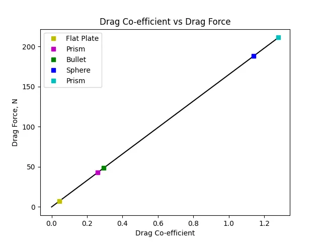
The curve obtained in Drag force vs Drag co-efficient is a straight line which is obvious since drag force is directly proportional to drag co-efficient. The drag co-efficient is depended on the shape irrespective of the frontal area, ie., the drag co-efficient is different for different shapes even though the frontal area is same.
From the graph, it shows that the drag force is minimum for aerofoil shape followed by sphere, bullet, prism and flat plate. So in order to reduce the drag force, the shape should be opted corresponding to the lower drag co-efficient. That is, shape does play an important role in producing drag force.
Conclusion
The PYTHON program to compute the Drag force has been successfully created. The velocity vs drag force and drag co-efficient vs drag force have been successfully plotted using the program and the variation of the graphs have been studied.
Reference
[1] https://www.trainingpeaks.com/blog/understanding-rolling-resistance/