SOLIDWORKS CFD Project: Transient Flow Over a Cylinder
Aim
To simulate the transient flow over a cylinder and create animations for pressure and velocity for the different Reynolds number.
Theory
External flow over objects is very important in Computational fluid dynamics because of the existing many practical applications. For instance, consider the case of an airfoil made of streamlined shape. Here, the main purpose of the airfoil shape is to increase the lifts and parallelly, to reduce the aerodynamic drags. On the other hand, if we consider the case of a cylinder (blunt body), there exist a boundary layer separation and very strong oscillations (eddies) in the wake region behind the body [1].
Due to the presence of the fluid viscosity, the fluid particles close to the solid surface would slow down and forms a thin slow-moving fluid layer called a boundary layer. To satisfy the no-slip condition at the surface, the flow velocity at the surface is zero. Inside the boundary layer, the flow momentum is quite low since it experiences a strong viscous flow resistance. This implies that, the boundary layer flow is sensitive to the external pressure gradient.
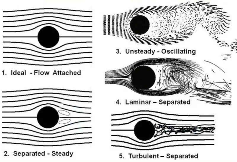
Figure 1: Flow Over a Cylinder [2]
Here, the transient flow of the fluid is studied. That is, the flow parameters such as velocity and pressure of the fluid particle changes with the time and position [3].
The Reynolds number is an important dimensionless quantity in fluid mechanics that helps in predicting the flow patterns of the different fluid flow situations. Reynolds number can reveal whether a flow is laminar and turbulent. At low Reynolds number, the flow tends to be dominated by the laminar flow, whereas at high Reynolds number, turbulence results from differences in the fluid's speed and direction. The transition from laminar to turbulent flow depends on the flow velocity, geometry, surface roughness, surface temperature and type of flow.
Reynolds number, `Re=(rho*v*d)/mu`
where, `rho` is the density of the fluid, `d` is the characteristic dimension of the pipe, `mu` is the dynamic viscosity of the fluid and `v` is the velocity of the fluid.
Objectives
- Understanding the transient flow and the basics of computational fluid dynamics.
- Simulate a transient flow over a cylinder.
- Find the corresponding Reynolds number and incrementing the Reynolds number as factor of 20%, 40% and 100% as different cases.
- Find corresponding velocity and simulation end time for each case.
- Simulation for each case and making animation for pressure and velocity contours.
- Comparing the flow of each case with the result and understanding the flow.
Procedure
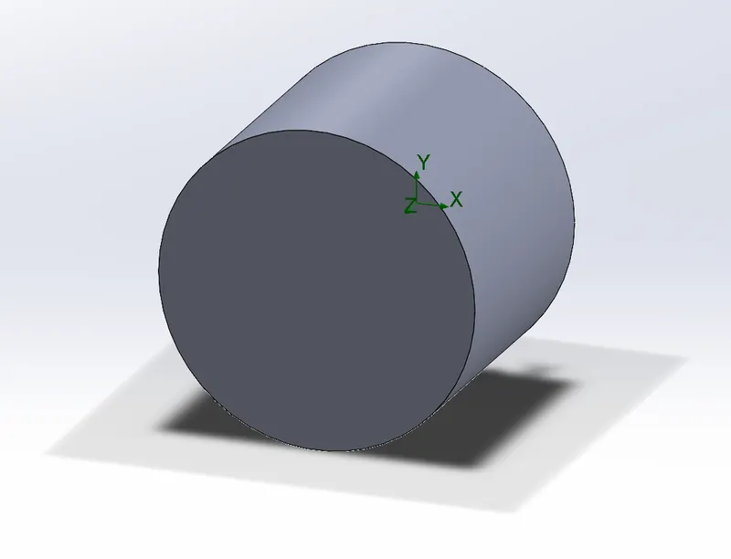
Here, the fluid is assumed to be air. Therefore, at 15 `°C`, the density of the fluid is `1.225 (kg)/m^3` and dynamic viscosity to be `1.81*10^-5 (kg)/(m.s)`. For this study, we are not considering the surface roughness and the temperature is at room temperature. The gravity is also neglected, and the pressure taken is the atmospheric pressure. The dimensions of the cylinder are, diameter, `d=15 mm=0.015m` and length, `l=25mm = 0.025m`.
From the Reynolds number equation, `v=(Re*mu)/(rho*d)`.
For the baseline simulation, we are considering the velocity, `v = 20 m/s`.
Therefore, Reynolds number, `Re = (rho*v*d)/mu = (1.225*20*0.015)/(1.81*10^-5) = 20303.8674`.
The Reynolds number is then increased by a factor of 20%, 40%, and 100% for the simulation to analyze the difference in the flow. The study is divided into 3 cases for each increment cases and it is compared to the baseline simulation.
From the Reynolds equation, Velocity, `v=(Re*mu)/(rho*d)`.
For the transient flow study, the simulation end time should be calculated properly. We need to consider the domain of study dimension for calculating the time requirement for the study. For the cylinder with `0.015 m` diameter, the computational domain considered is `0.15 m`along the x direction, `0.12m` along the y direction and `0.08 m` along the z direction for the length of the cylinder, `0.025m`. For calculating the required time for simulation, we need to know the time required by the fluid from the inlet of the domain to reach the exit of the domain. Here, the flow is to take place along the x direction, that is, we need to consider the length of domain along x direction and equating it with the velocity of the fluid, the flow through time can be calculated. The flow through time is to be multiplied with 2, to the get the simulation end time, to make sure the flow has enough time and to evaluate the effect of the flow. For the calculation in this problem, the flow through time is multiplied with 2.5 as a factor of safety to increase the analysis/simulation time.
For Baseline Simulation
Velocity, `v=20m/s`.
Reynolds number, `Re=20303.8674`
Flow through time = computational domain length / velocity = `0.15/20 = 7.5*10^-3 s`
Simulation end time = `0.01875 s`
Flow the flow simulation, external flow is chosen, and the time dependent is checked to make the simulation transient study. The total analysis time is set as `0.01875 s` which is calculated as simulation end time. The output time step is set as 0.00125 to have 15 evaluations points between 0.01875 s.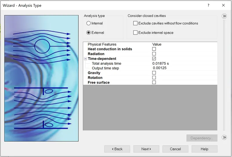
The chosen fluid for the study is air.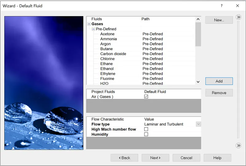
Since the flow is considered only along the x direction and is taken to be `20 m/s`, the velocity along the x direction is provided.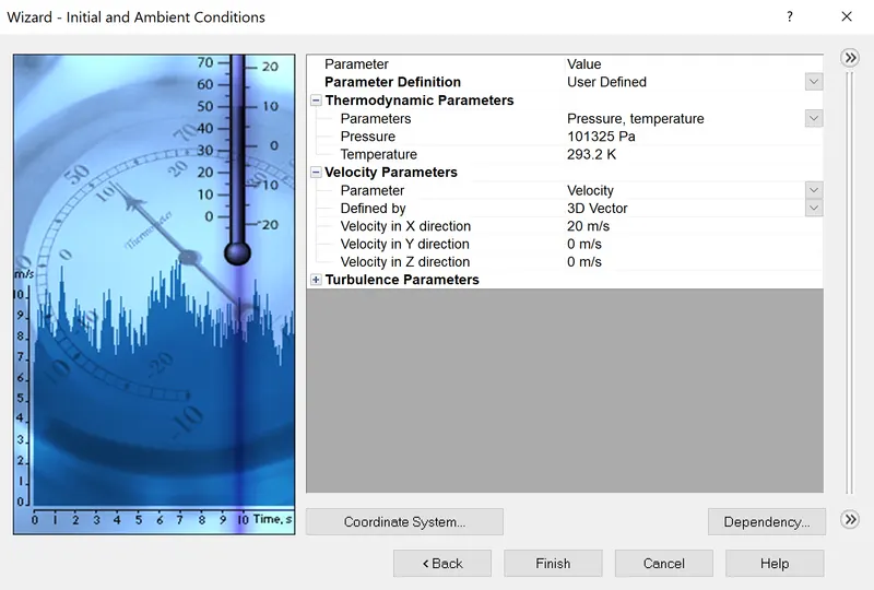
The Solidworks will provide the computational domain for the simulation study as default, but it is edited to make sure that it has the limit within the required range as mentioned above for calculating the simulation end time.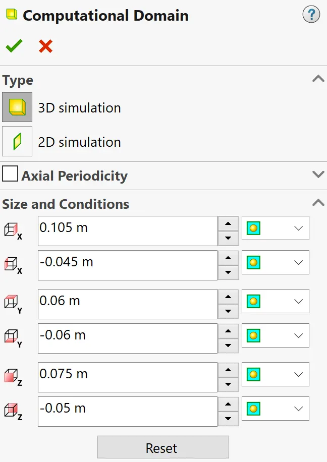
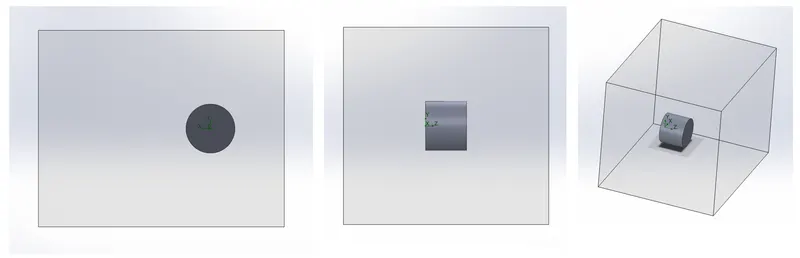
Now, the simulation is done, and the corresponding velocity and pressure animation is made.
The velocity plot is: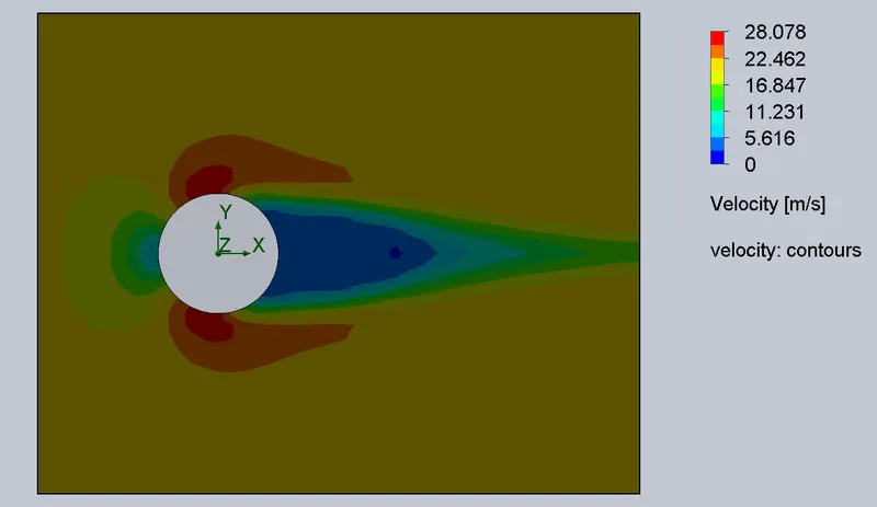
The pressure plot is: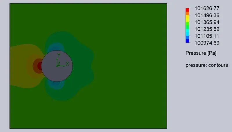
The animation of the transient flow is:
- Velocity
- Pressure
Case 1: 20% increment in Reynolds Number
Reynold number is, `Re=24364.64`.
Corresponding velocity, `v=24m/s`
Flow through time = `6.25*10^-3 s`
Simulation end time = `0.015625 s`
Output step time = `0.001041666 s`
The simulation is then run for the above velocity with all other parameter been set as same and the corresponding velocity and pressure animations are made.
The velocity plot is: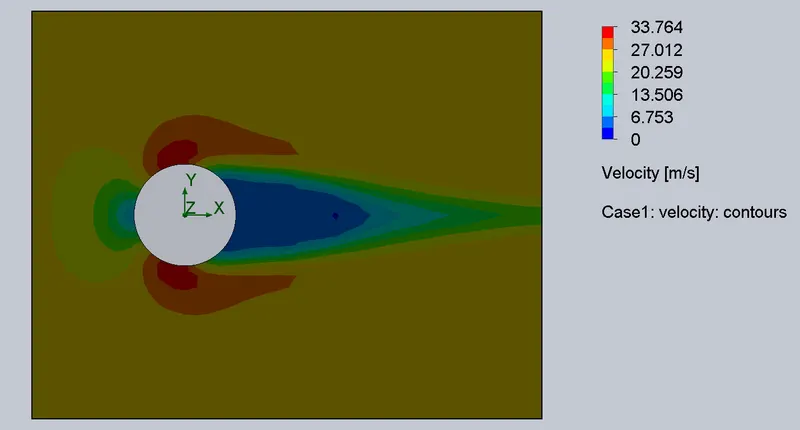
The pressure plot is: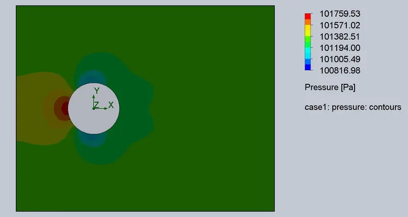
The animation of the transient flow is:
- Velocity
- Pressure
Case 2: 40% increment in Reynolds Number
Reynold number is, `Re=28425.41436`.
Corresponding velocity, `v=28 m/s`
Flow through time = `5.357142858*10^-3 s`
Simulation end time = `0.01339285715 s`
Output step time = `0.000892857 s`
The simulation is then run for the above velocity with all other parameter been set as same and the corresponding velocity and pressure animations are made.
The velocity plot is: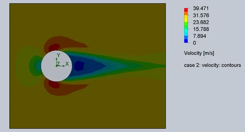
The pressure plot is: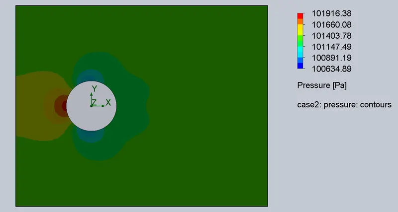
The animation of the transient flow is:
- Velocity
- Pressure
Case 3: 100% increment in Reynolds Number
Reynold number is, `Re=40607.7348`.
Corresponding velocity, `v=40 m/s`
Flow through time = `3.77*10^-3 s`
Simulation end time = `0.009375 s`
Output step time = `0.000625 s`
The simulation is then run for the above velocity with all other parameter been set as same and the corresponding velocity and pressure animations are made.
The velocity plot is: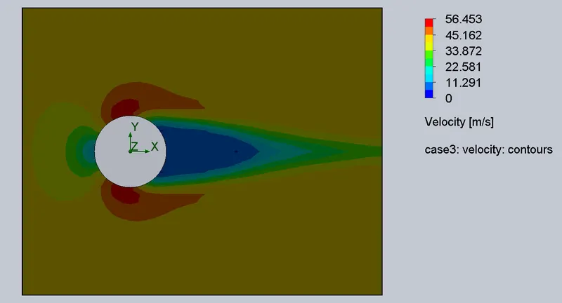
The pressure plot is: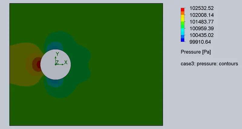
The animation of the transient flow is:
- Velocity
- Pressure
Conclusion
With the increase in the Reynolds number, the velocity of the external flow will also increase, hence the time required for the flow to complete over the domain decreases. That is, the required time to obtain the velocity and pressure profile will decrease. As the Reynolds number is increased, the steadiness of the flow decreases, that is, the flow would become turbulent.
At higher velocities, the boundary layer is formed, at the region behind the cylinder (Separation region).
Reference
[1] http://eng-web1.eng.famu.fsu.edu/~shih/succeed/cylinder/cylinder.htm
[2] https://www.grc.nasa.gov/www/k-12/airplane/dragsphere.html
[3] https://www.gunt.de/en/products/fluid-mechanics/transient-flow/glct-1:pa-148:ca-781#:~:text=Transient%20flow%3A%20the%20velocity%20of,Transient%20flow%3A%20experimental%20units