MATLAB Project: Curve Fitting
Aim
To write MATLAB code to fit a linear and cubic polynomial for the Cp data, and plot the linear and cubic fit curves along the raw data points.
Theory
Curve fitting is the process of constructing a curve, or mathematical function, that has the best fit to a series of data points, possibly subject to constraints [1]. It can be either interpolation, where an exact fit to the data is required, or smoothing, where a smooth function is constructed that approximately fits the data. By curve fitting, we can mathematically construct the functional relationship between the observed data set and parameters values, etc [2]. It is highly effective in mathematical modeling of some natural processes [3].
For understanding more about curve fitting [2], assume as set of data points `(x_1,y_1), (x_2,y_2), (x_3,y_3), ... ,`and `(x_n,y_n)`. Let `y=f(x)` be the best fit for these set of points.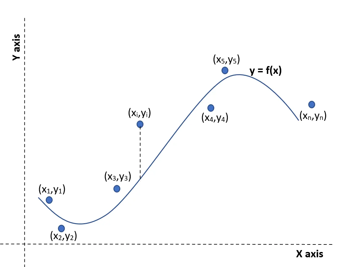
Since these data points doesn't really lie exactly on the function curve, there exist a error for each data points. The general expression for error of the data point (`x_i,y_i`) is,
`Err_i`=|`y_i``-` value of `f(x)` at `x_i`| = |`y_i - f(x_i)`|
The error term is squared in order to have an effect of removal of modulus sign. That is,
SSE (sum of squared errors)=`sum_(i=1)^n Err_i^2`
Assume the equation is in nth degree polynomial of the form,
`f(x)=A_1+A_2*x+A_3*x^2+...+A_n*x^(n-1)`
For finding the minima and the value of coefficient, we differentiate SSE with each and every coefficient of the proposed equation `f(x)` and equating it to zero, we get,
`[[(∂SSE)/(∂A_1) = 0],[(∂SSE)/(∂A_2) = 0],[.],[.],[.],[(∂SSE)/(∂A_n)=0]]`
by solving, we get the values of all the coefficients. This method is known as Least Square Method is the most commonly used technique. This method can be used to measure the goodness of the fit criteria or how wee the equation is representing the data points.
SSE value minimum (close to zero) means better the curve fit.
Similarly, there are other methods to evaluate the goodness of fit including R-square, Adjusted R-square and Root mean squared error (RMSE).
R-square can be calculated using the following formula,
`R^2=(SSR)/(SSE)`
where, SSE is the sum of squares due to error and SSR is the squares of regression (square of the difference between the value of the fitting function at a given point and the arithmatic mean of the data set).
`SSR=sum_(i=1)^n(f(x_i)-Mean)^2`
`SST=SSR+SSE`
The higher the value of R-square, the better the fit. The R-square can ranges from a value of 0 to 1.
Root Mean Squared Error (RSME) is also known as the fit standard error and the standard error of the regression. It is an estimate of the standard deviation of the random component in the data and is defined as,
`RMSE=sqrt((SSE)/n)`
where, n is the total number of datapoints available.
- Using these quantities, the goodness of the fit can be understood. For R-square greater than 0.95, the fit is assumed to be good.
Objectives
- Understanding the theoretical concepts of Curve fitting.
- Writing a program in MATLAB to fit a linear and cubic polynomial for the Cp data.
- Understanding the parameters used to measure the fitness characteristics for both the curves.
- Writing a code in MATLAB to show splitwise method.
- Understating the Curve fitting toolbox in MATLAB and using it.
- Answering the questions on Curve fit.
Program to plot Original, Linear, Quadratic and Cubic Curve
The programming is done in MATLAB.
clear all
close all
clc

% Preparing data
cp_data = load('data');
temperature = cp_data(:,1);
cp = cp_data(:,2);

% Plot Original Values
figure (1)
plot(temperature,cp);
xlabel('Temperature [K]');
ylabel('Specific Heat [kJ/kmol-K]');
title('Original Curve Fit');
grid on;
grid minor;

% For plotting linear curve fit
% function, cp2 = p1*x + p2

p_1 = polyfit(temperature,cp,1);
cp_1 = polyval(p_1,temperature);

sse1 = 0; % initialising sse1 to 0
ssr1 = 0; % initialising sse1 to 0
error1 = cp - cp_1; % Calculating error
error1_sqr = error1.^2; % Squaring the error
mean1 = mean(cp_1); % calculating mean
error1_r = cp_1 - mean1; % for calculating ssr
error1_r_sqr = error1_r.^2;
% for loop for adding each element of matrix
for i = 1:length(cp)

    sse1 = sse1 + error1_sqr(i);
    ssr1 = ssr1 + error1_r_sqr(i);

end
error1_m = abs(error1); % finding the absolute value
sst1 = ssr1 + sse1; % calculating sst

figure (2)

subplot(8,3,[1:15]) % for plotting linear and original curve fit
plot(temperature,cp_1,'color','r');
hold on;
plot(temperature,cp,'color','b');
hold off;
xlabel('Temperature [K]');
ylabel('Specific Heat [kJ/kmol-K]');
title('Linear vs Original Curve Fit');
legend('Linear curve fit','Original curve fit');
axis([300 3500 900 1400]);
grid on;
grid minor;

subplot(8,3,[19:24]) % for plotting error curve
plot(temperature,error1_m,'color','k');
xlabel('Temperature [K]');
ylabel('Absolute Error Value');
title('Error Curve');
axis([300 3500 0 100]);
grid on;
grid minor;


% For plotting quadratic curve fit
% function, cp1 = p1*x^2 + p2*x + p3

p_2 = polyfit(temperature,cp,2);
cp_2 = polyval(p_2,temperature);

sse2 = 0; % initialing value
ssr2 = 0; % initialising value
error2 = cp - cp_2; % calculating error
error2_sqr = error2.^2; % squaring the error value
mean2 = mean(cp_2); % finding mean
error2_r = cp_2 - mean2; % for calculating ssr
error2_r_sqr = error2_r.^2; % squaring each term
for i = 1:length(cp) % for loop to add each term of the vector

    sse2 = sse2 + error2_sqr(i);
    ssr2 = ssr2 + error2_r_sqr(i);

end
error2_m = abs(error2); % finding absolute value
sst2 = ssr2 + sse2; % calculating sst

figure (3)

subplot(8,3,[1:15]) % for plotting original and quadratic curve
plot(temperature,cp_2,'color','r');
hold on;
plot(temperature,cp,'color','b');
hold off;
xlabel('Temperature [K]');
ylabel('Specific Heat [kJ/kmol-K]');
title('Quadratic vs Original Curve Fit');
legend('Quadratic curve fit','Original curve fit');
axis([300 3500 900 1400]);
grid on;
grid minor;

subplot(8,3,[19:24]) % for calculating error curve
plot(temperature,error2_m,'color','k');
xlabel('Temperature [K]');
ylabel('Absolute Error Value');
title('Error Curve');
axis([300 3500 0 100]);
grid on;
grid minor;

% For plotting cubic curve fit
% function, cp3 = p1*x^3 + p2*x^2 + p3*x + p4

[p_3,s,mu] = polyfit(temperature,cp,3);
cp_3 = polyval(p_3,temperature,s,mu);

sse3 = 0; % initialising value
ssr3 = 0; % initialising value
error3 = cp - cp_3; % calculating error
error3_sqr = error3.^2; % squaring error value
mean3 = mean(cp_3); % calculating mean
error3_r = cp_3 - mean1; % for calculating ssr
error3_r_sqr = error3_r.^2; % for squaring
for i = 1:length(cp) % for loop to add each term

    sse3 = sse3 + error3_sqr(i);
    ssr3 = ssr3 + error3_r_sqr(i);

end
error3_m = abs(error3); % finding absolute value
sst3 = ssr3 + sse3; % calculating sst

figure (4)

subplot(8,3,[1:15]) % for plotting cubic and original curve fot
plot(temperature,cp_3,'color','r');
hold on;
plot(temperature,cp,'color','b');
hold off;
xlabel('Temperature [K]');
ylabel('Specific Heat [kJ/kmol-K]');
title('Cubic vs Original Curve Fit');
legend('Cubic curve fit','Original curve fit');
axis([300 3500 900 1400]);
grid on;
grid minor;

subplot(8,3,[19:24]) % for plotting error curve
plot(temperature,error3_m,'color','k');
xlabel('Temperature [K]');
ylabel('Absolute Error Value');
title('Error Curve');
axis([300 3500 0 100]);
grid on;
grid minor;

% Calculating SSE, R-square and RMSE for choosing best fit
n = length(temperature); % number of data points for calculating RMSE

% For Linear curve fit
SSE1 = sse1; % SSE
R_square1 = ssr1/sst1; % R-square
RMSE1 = (sse1/n)^(0.5); % RSME

% For Quadratic curve fit
SSE2 = sse2; % SSE
R_square2 = ssr2/sst2; % R-square
RMSE2 = (sse2/n)^(0.5); % RSME

% For Cubic curve fit
SSE3 = sse3; % SSE
R_square3 = ssr3/sst3; % R-square
RMSE3 = (sse3/n)^(0.5); % RSME

% creating Table
Curve_Fit = {'Linear';'Quadratic';'Cubic'};
SSE = [SSE1;SSE2;SSE3];
R_Square = [R_square1;R_square2;R_square3];
RMSE = [RMSE1;RMSE2;RMSE3];

table(SSE,R_Square,RMSE,'RowNames',Curve_Fit)

%Comparison of Curve fit and error
figure (5)
subplot(8,3,[1:15])
plot(temperature,cp,'color','k','linewidth',1);
hold on;
plot(temperature,cp_1,'color','b','linewidth',1);
hold on;
plot(temperature,cp_2,'color','r','linewidth',1);
hold on;
plot(temperature,cp_3,'color','g','linewidth',1);
hold off;
xlabel('Temperature [K]');
ylabel('Specific Heat [kJ/kmol-K]');
title('Curve Fit Comparison');
legend('Original','Linear','Quadratic','Cubic');
axis([300 3500 900 1400]);
grid on;
grid minor;

subplot(8,3,[19:24])
plot(temperature,error1_m,'color','b','linewidth',1);
hold on;
plot(temperature,error2_m,'color','r','linewidth',1);
hold on;
plot(temperature,error3_m,'color','g','linewidth',1);
hold off;
axis([0 3400 0 150]);
xlabel('Temperature [K]');
ylabel('Absolute Error value');
legend('Linear','Quadratic','Cubic');
title('Error Comparison');
grid on;
grid minor;
Each step of the program is explained with comments. The data file loaded in the program consist of temperature and specific heat values in the respective first and second column.
p = polyfit(x,y,n) command returns the coefficients for a polynomial p(x) of the degree n that is a best fit (in a least-square sense) for the data in y [4]. y = polyval(p,x) returns the value of a polynomial of degree n evaluated at x. The input p is a vector of length n+1 whose elements are the coefficient in descending powers of the polynomial value [5].
table command is used to create table where the 'RowName' makes that particular column not a table variable, but instead a property of the table [6].
If we have used p = polyfit(x,y,n) comand for cubic curve it, it would have shown a error as below:
p = polyfit(x,y,n) only returns the coefficient of the a polynomial p(x). Instead, if we use [p,s,mu] = polyfit(x,y,n), then it would returns a structure s and mu. The structure s can be used as an input to polyval to obtain error estimate. mu is a two-element vector with centering and scaling values. mu(1) is mean(x) and mu(2) is std(x). By using these values, polyfit centers x at zero nad scales it to have unit standard deviation. Therefore, by using [p,s,mu] = polyfit(x,y,n), the above shown warning can be removed as this centering and scaling transformation improves the numerical properties of both the polynomial and the fitting algorithm.
Output of the program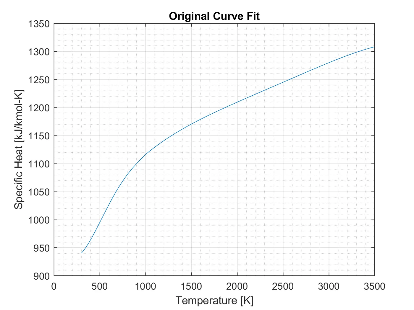
Figure 1: Original Curve Fit
The Figure 1 shows the graph plot between the values found in the file 'data'. This is the actual values of specific heat with respect to the temperature. The curves formed by Linear, Quadratic and Cubic polynomial fit will be compared to this graph to understand the accuracy or the best fit of the respective curve fits.
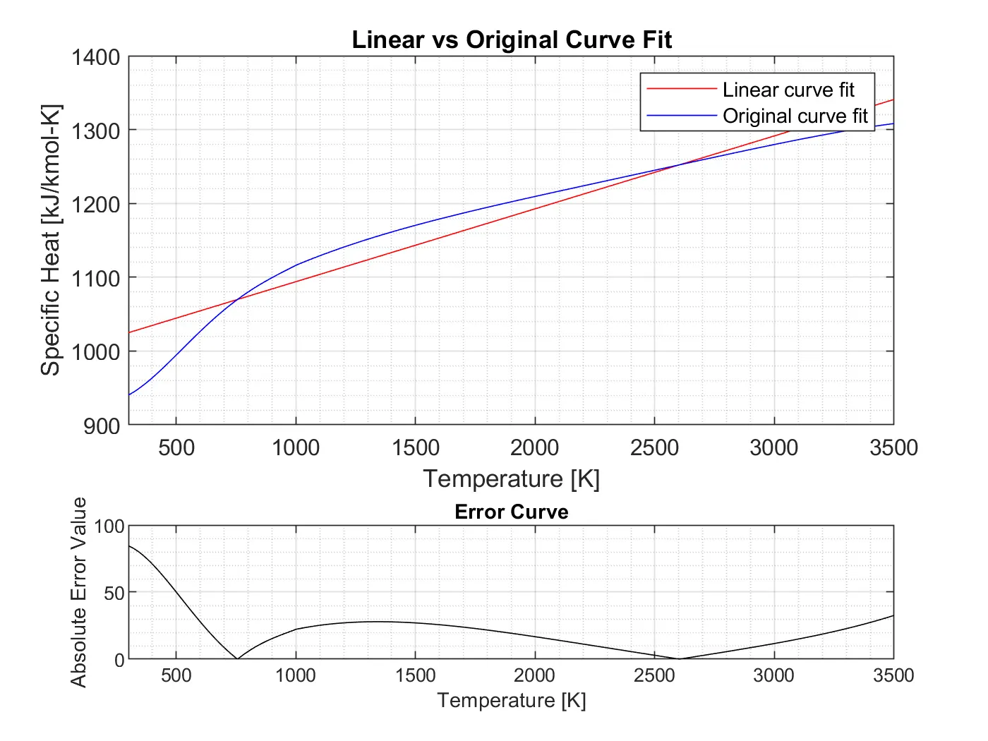
Figure 2: Linear curve fit and its error curve
Figure 2 represents the Linear curve fit along with raw data. The error curve below represents the deviation of specific heat value formed by the linear curve fit from the original value at each value of temperature.
Similarly, the Figure 2 and Figure 3 shows the quadratic and cubic curve fits alon with the raw data and its corresponding error curves.
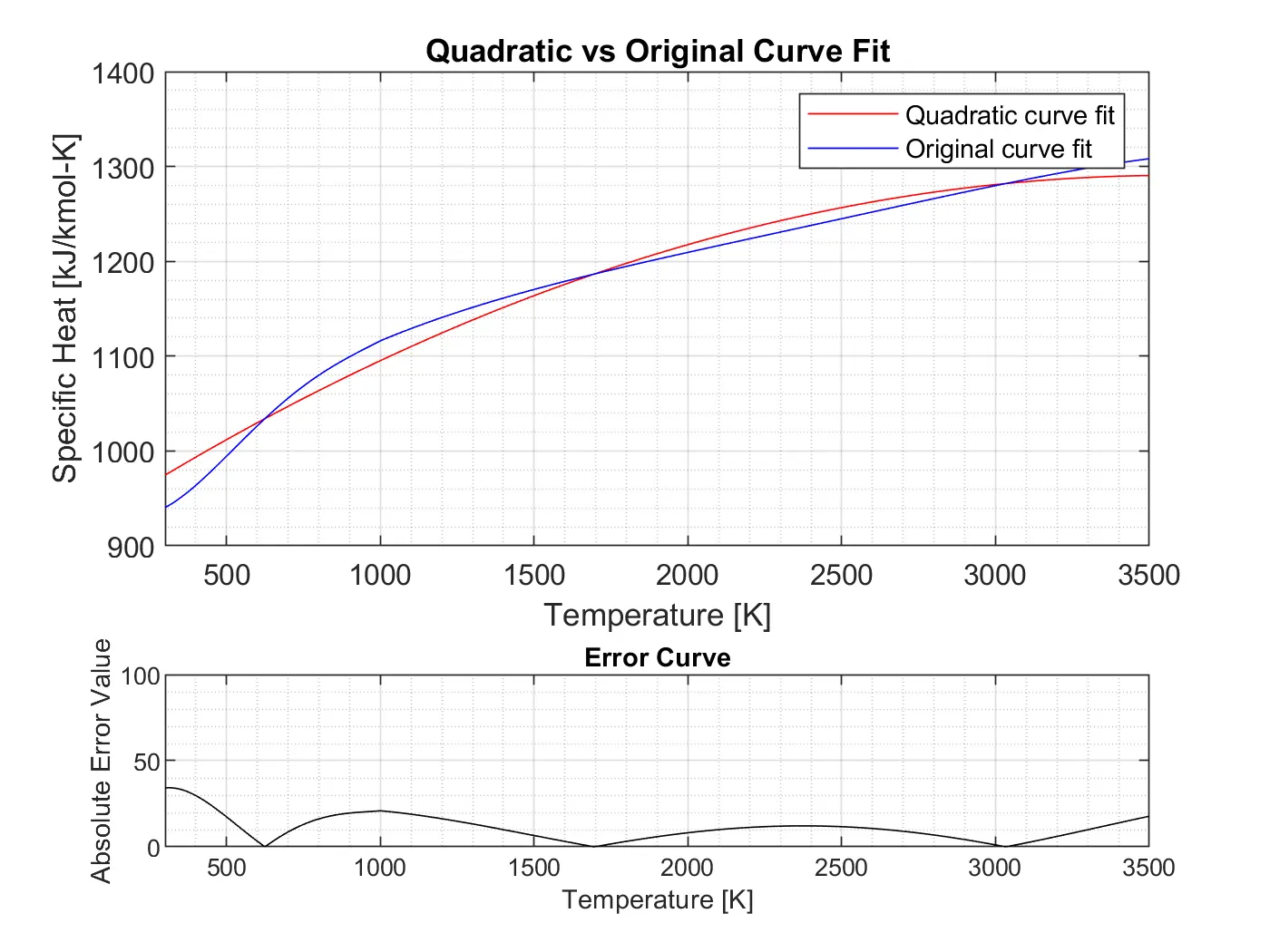
Figure 3: Quadratic curve fit and its error curve
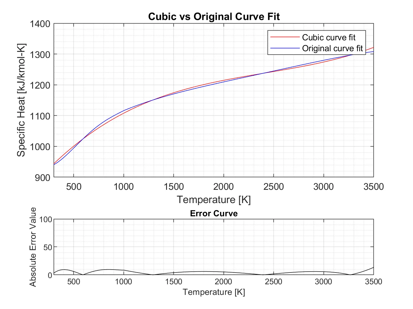
Figure 4: Cubic curve fit and its error curve
Figure 4 depicts the Cubic curve fit and its error curve. This curve seems to fit more properly than the other two curves.
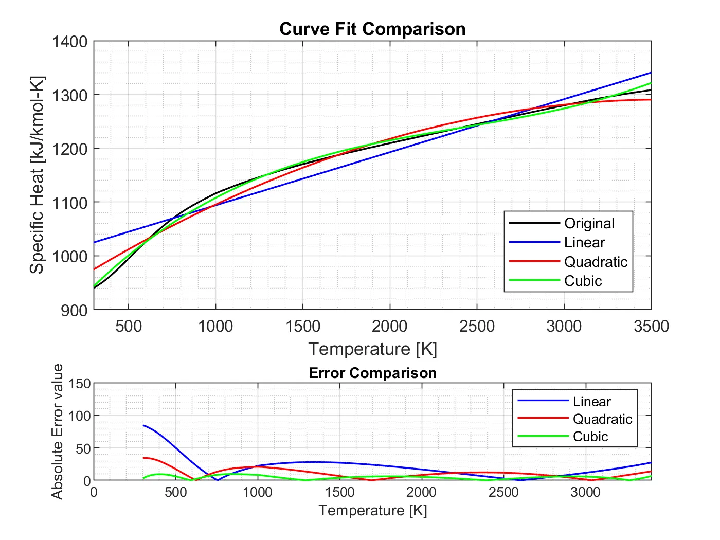
Figure 5: Comparison of fit curves
Figure 5 depicts the graph plotted for comparison of each linear, quadratic as well as cubic fit curves with respect to the original values. From the graph, it is clear that the cubic fit curve has more accurate value than the other two curves followed by quadratic and linear fit curves respectively. To understand more, the error curve gives more idea where it represents the absolute value of error for all three curves at each point temperature points. It is observed that the cubic curve fit has comparatively lesser error value than other followed by quadratic and linear. For knowing the absolute value of maximum error for each curve fit, refer figure 6. The maximum value of error found for linear curve fit is 84.4621 units while for quadratic curve fit, its maximum error value is 34.2904 which is huge development than from the linear curve fit and the minimum error is seen for cubic curve fits, where its maximum error value is only 13.4401 units.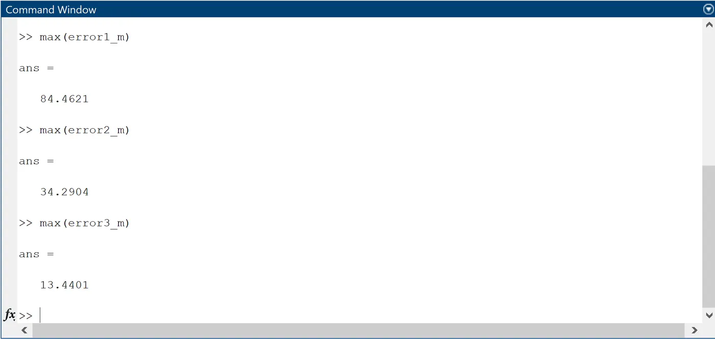
Figure 6: Maximum value of error for each curve fit.
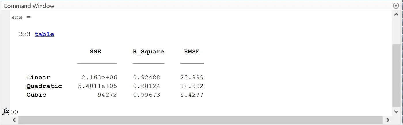
Figure 7: SSE, R-square and RMSE value of linear, quadratic and cubic curves
Figure 7 represents the SSE, R-square and RMSE values for the linear, quadratic and cubic curve fit. These values are used to find the best fit, that is, goodness of the fit or how well the equation is representing the datapoints. If the R-square is greater than 0.95, the fit is assumed to be good. Here, quadratic as well as cubic curve fits have R-square value greater than 0.95 which means that the linear curve fit here is not good. Since the value of R-square for cubic curve fit is more closer to 1 than quadratic, implies that cubic curve fit here is better compared to other two.
Program to show Splitwise method
In this method we split the data into multiple sets so as to have better curve fit. For eliminating the error, we have to use centering and scaling by using code. The given data file contains temperature value ranging from 300 to 3499, that is 3200 elements. Here, for splitwise method, the temperature set is divided into four sets and each set is calculated assumed to be polynomial function with different degree.
- Element 1 to 640: Set 1
- Element 641 to 1280: Set 2
- Element 1281 to 1920: Set 3
- Element 1921 to 2560: Set 4
- Element 2561 to 3200: Set 5
The programming is done in MATLAB.
clear all
close all
clc

% Preparing data
cp_data = load('data');
temperature = cp_data(:,1);
cp = cp_data(:,2);

% dividing temperature into 5 sets
temperature1 = temperature([1:640]);
temperature2 = temperature([641:1280]);
temperature3 = temperature([1281:1920]);
temperature4 = temperature([1921:2560]);
temperature5 = temperature([2561:3200]);

% dividing cp into 5 sets
cp1 = cp([1:640]);
cp2 = cp([641:1280]);
cp3 = cp([1281:1920]);
cp4 = cp([1921:2560]);
cp5 = cp([2561:3200]);

% Curve fit for each set (order 3)
[p_1,s1,mu1] = polyfit(temperature1,cp1,3);
cp_1 = polyval(p_1,temperature1,s1,mu1);

[p_2,s2,mu2] = polyfit(temperature2,cp2,3);
cp_2 = polyval(p_2,temperature2,s2,mu2);

[p_3,s3,mu3] = polyfit(temperature3,cp3,3);
cp_3 = polyval(p_3,temperature3,s3,mu3);

[p_4,s4,mu4] = polyfit(temperature4,cp4,3);
cp_4 = polyval(p_4,temperature4,s4,mu4);

[p_5,s5,mu5] = polyfit(temperature5,cp5,3);
cp_5 = polyval(p_5,temperature5,s5,mu5);

% Plotting Curve
plot(temperature,cp,'color','k','linewidth',1);
hold on;
plot(temperature2,cp_2,'color','r','linewidth',1);
hold on;
plot(temperature3,cp_3,'color','y','linewidth',1);
hold on;
plot(temperature4,cp_4,'color','m','linewidth',1);
hold on;
plot(temperature5,cp_5,'color','g','linewidth',1);
hold on;
plot(temperature1,cp_1,'color','b','linewidth',1);
hold off;
grid on;
grid minor;
xlabel('Temperature [K]');
ylabel('Specific Heat [kJ/kmol-K]');
title('Split wise');
legend('Original','Set 1','Set 2','Set 3','Set 4','Set 5');
Output of the program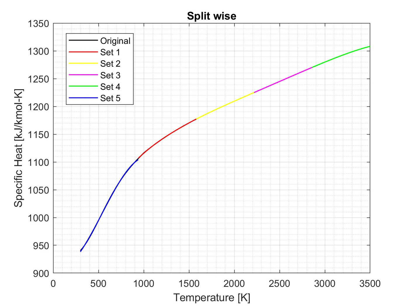
The output plot of the splitwise program is shown above.
Using Curve Fitting Toolbox in MATLAB
In curve fitting toolbox, we don't use any curve fit functions like 'polyfit' or 'polyval' and can mention the datasets directly under the X data and Y data option. The advantage of the toolbox is that it enables to perform fitting of 3d surfaces too, which cannot be seen in 'polyfit'. The fitting techniques commonly used are interpolant and polynomial for the unknown nature of experimental data. Fourier is used to fit data which is similar to waveforms. 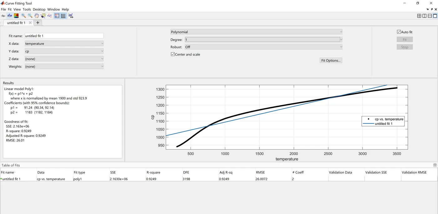
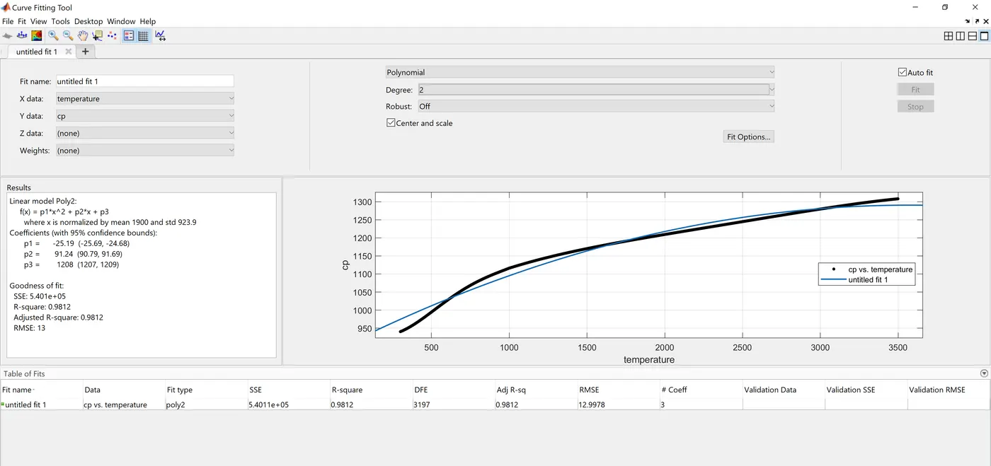
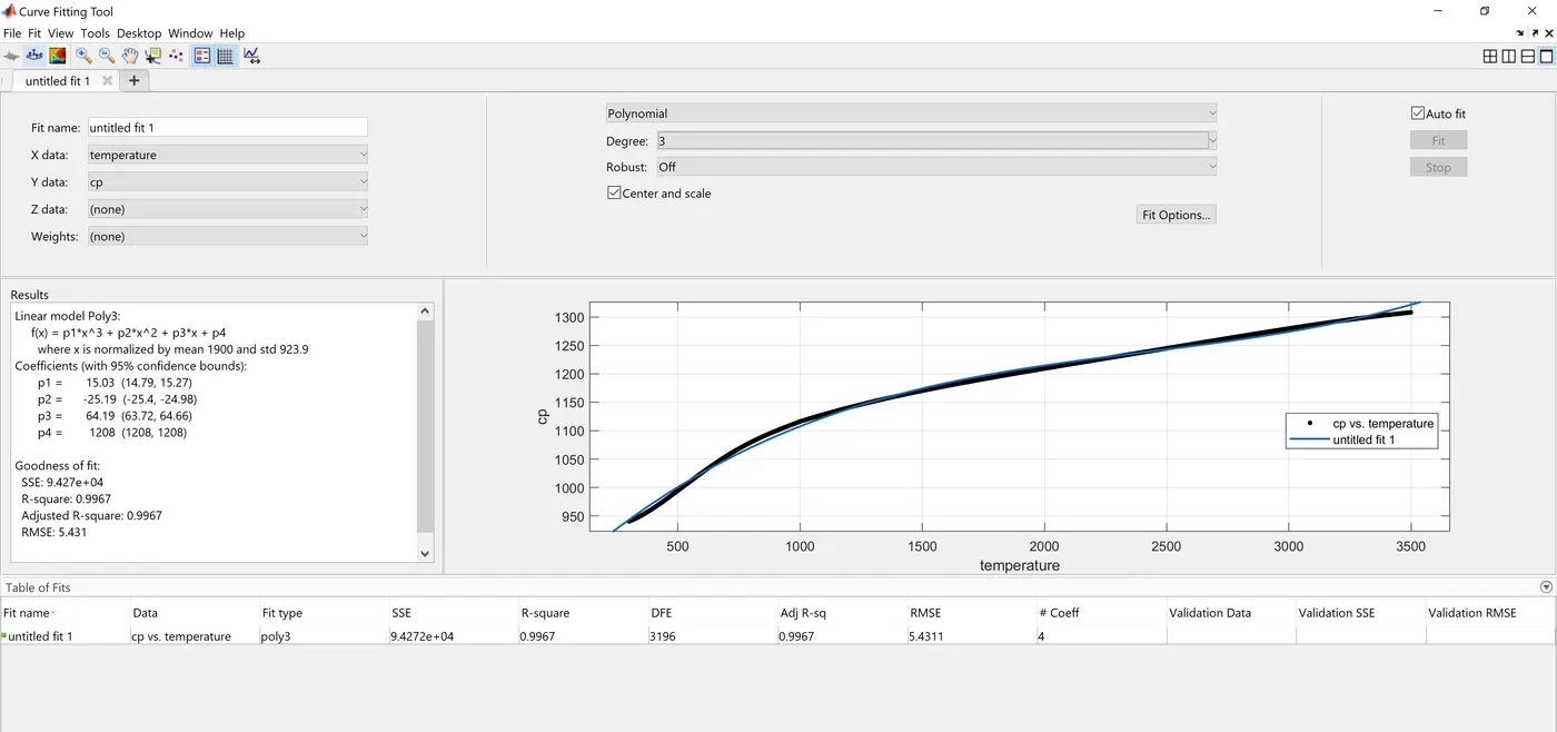
The above are the screenshots of the curve fitting for linear (degree:1), quadratic (degree:2) and cubic (degree:3) polynomials. The goodness of the plot will be evaluated automatically by the toolbox which is shown in the result section (left side) of the toolbox. The SSE, R-square and RSME value that we found for linear, quadratic and cubic manually are found to be same which is calculated by the toolbox automatically. This reveals that, the manual calculation is right.
Question answer
How to make a curve fit perfectly?
The curve that gives zero error between data y and the fit f(x) is the perfect fit. If the curve fit perfectly, then the R-square of the curve will equals one. Also, for perfect fit curve, the SSE quantity will be zero. The curve fit should match with the original data without showing the error in the command window. In order for setting the curve perfectly, we can eliminate the error by using the center and scaling code that is by elimination of error.
How to get the best fit? Note: Best fit and perfect fit are two completely different phenomena.
Consider the general form for a polynomial of order j
`f(x)=a_0+a_1x+a_2x^2+a_3x^3+...+a_jx^j=a_0+sum_(k=0)^ja_kx^k`. Let this be the equation for the curve fit. The curve that gives minimum error between data y and the fit f(x) is the best fit.
The best fit can be obtained by increasing the order of the polynomial and also by splitting the curves into multiple range and then plotting for each range set.
There are different methods to understand the goodness of the curve fit, namely he sum of squares due to error (SSE), R-square, Adjusted R-square and Root mean squared error (RMSE). From these quantities, we can evaluate the best fit of the curve.
What could be done to improve the cubic fit?
For improving the cubic fit, the splitwise method can be used where the data set in divided into multiple range. More the division, more will be the improvement to the curve.
Conclusion
The MATLAB program to fit a linear, quadratic and cubic polynomial for the Cp data has been created successfully and has been plotted along with the raw data. The parameters such as SSE, R-square, Adjusted R-square and RMSE to measure the fitness characteristics of the curves has been understood and found.
The MATLAB code to show splitwise method has been created and the output plot of the curve is found and understood. The MATLAB Curve fitting toolbox to validate the fitness characteristics has been understood and the corresponding value obtained has been compared with value obtained manually.
References
[1]https://en.wikipedia.org/wiki/Curve_fitting
[2]https://skill-lync.com/projects/Curve-Fitting-and-criterion-to-choose-best-fit-41860
[3]https://ncss-wpengine.netdna-ssl.com/wp-content/themes/ncss/pdf/Procedures/NCSS/Introduction_to_Curve_Fitting.pdf
[4]https://www.iiserpune.ac.in/~bhasbapat/phy221_files/curvefitting.pdf
[5]https://statisticsbyjim.com/regression/curve-fitting-linear-nonlinear-regression/
[6]https://in.mathworks.com/help/matlab/ref/table.html
[7]https://in.mathworks.com/help/matlab/ref/polyfit.html