PYTHON Project: Curve Fitting
Aim
To write PYTHON code to fit a linear and cubic polynomial for the Cp data and plot the linear and cubic fit curves along the raw data points.
Theory
Curve fitting is the process of constructing a curve, or mathematical function, that has the best fit to a series of data points, possibly subject to constraints [1]. It can be either interpolation, where an exact fit to the data is required, or smoothing, where a smooth function is constructed that approximately fits the data. By curve fitting, we can mathematically construct the functional relationship between the observed data set and parameters values, etc [2]. It is highly effective in mathematical modeling of some natural processes [3].
For understanding more about curve fitting [2], assume as set of data points `(x_1,y_1),(x_2,y_2),(x_3,y_3)`, ...., and `(x_n,y_n)`. Let `y=f(x)` be the best fit for these set of points.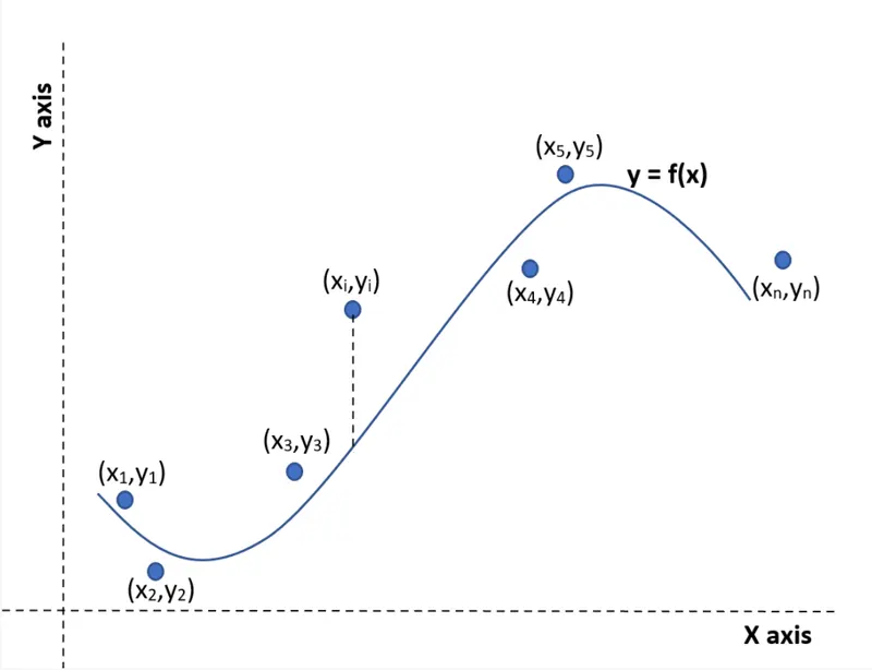
Since these data points doesn't really lie exactly on the function curve, there exist an error for each data points. The general expression for error of the data point `(x_i,y_i)` is,
`Err_i = |y_i- "value of " f(x) " at "x_i| = |y_i-f(x_i)|`
The error term is squared in order to have an effect of removal of modulus sign. That is,
`SSE" (sum of squared errors)"=sum_(i=1)^nErr_i^2`
Assume the equation is in nth degree polynomial of the form,
`f(x)=A_1+A_2*x+A_3*x^2+...+A_n*x^(n-1)`
For finding the minima and the value of coefficient, we differentiate SSE with each and every coefficient of the proposed equation `f(x)` and equating it to zero, we get,
`[[(delSSE)/(delA_1)=0],[(delSSE)/(delA_2)=0],[.],[.],[.],[(delSSE)/(delA_n)=0]]`
by solving, we get the values of all the coefficients. This method is known as Least Square Method is the most commonly used technique. This method can be used to measure the goodness of the fit criteria or how wee the equation is representing the data points.
SSE value minimum (close to zero) means better the curve fit.
Similarly, there are other methods to evaluate the goodness of fit including R-square, Adjusted R-square and Root mean squared error (RMSE).
R-square can be calculated using the following formula,
`R^2=(SSR)/(SSE)`
where, SSE is the sum of squares due to error and SSR is the squares of regression (square of the difference between the value of the fitting function at a given point and the arithmetic mean of the data set).
`SSR=sum_(i=1)^n(f(x_i)-Mean)^2`
`SST = SSR+SSE`
The higher the value of R-square, the better the fit. The R-square can range from a value of 0 to 1.
Root Mean Squared Error (RSME) is also known as the fit standard error and the standard error of the regression. It is an estimate of the standard deviation of the random component in the data and is defined as,
`RMSE=sqrt((SSE)/n)`
where, n is the total number of datapoints available.
- Using these quantities, the goodness of the fit can be understood. For R-square greater than 0.95, the fit is assumed to be good.
Objectives
- Understanding the theoretical concepts of Curve Fitting.
- Exploring the typica PYTHON commands and functions for curve fitting such as popt, pcov, scipy.optimize, *popt, etc.
- Write a PYTHON code to fit linear and cubic polynomial for the Cp data.
- Measurment of how well the curve fits.
- Exploring the ways need to be done in order to make the curve fit perfectly.
Program to Plot Original, Linear and Cubic Polynomial Curve Fit
The programming is done in PYTHON.
# Program for Curve Fitting: Linear and Cubic Polynomial

import math
import matplotlib.pyplot as plt
import numpy as np
from scipy.optimize import curve_fit
from statistics import mean
from tabulate import tabulate


# Linear Fit Function
def func_linear(t,a,b):
	return (a*t)+b

# Cubic Fit Function
def func_cubic(t,a,b,c,d):
	return (a*pow(t,3))+(b*pow(t,2))+(c*t)+d


# Read thermodynamic data file
def read_file():
	temperature = []
	cp = []
	for line in open('data','r'): 	#each line with temp and cp value separated by comma is to be extracted
		values = line.split(',')	#extracted value need to converted into float data type
		temperature.append(float(values[0]))
		cp.append(float(values[1]))

	return [temperature,cp]


# Main Program
temperature, cp = read_file()

# Plot Original Data
plt.figure(1)
plt.plot(temperature,cp)	#ploting extracted temp and cp values
plt.xlabel('Temperature [K]')
plt.ylabel('Specific Heat [kJ/kmol-K]')
plt.title('Original Data')

# Linear Fit
popt, pcov = curve_fit(func_linear,temperature,cp)
fit_cp_linear = func_linear(np.array(temperature), *popt)

# Measurement of Fitness of Linear Fit
sse1 = 0	#initialising sse1 to 0
ssr1 = 0	#initialising ssr1 to 0
error1 = cp-fit_cp_linear			#calculating error
error1_sqr = pow(error1,2)			#squarring error
mean1 = mean(fit_cp_linear)			#calculating mean
error1_r = fit_cp_linear - mean1	#for calculating ssr
error1_r_sqr = pow(error1_r,2)

# for loop used to add each element
for i in range(0,len(cp)):
	sse1 = sse1+error1_sqr[i]
	ssr1 = ssr1+error1_r_sqr[i]

error1_m = abs(error1)				#finding absolute value
sst1 = ssr1+sse1					#calculating sst

# Plotting
plt.figure(2)
grid = plt.GridSpec(3, 1, wspace=0.4, hspace=0.3)
plt.subplot(grid[:2, 0])
plt.plot(temperature,cp,'b--')
plt.plot(temperature,fit_cp_linear,'r')
plt.legend(['Actual Data','Linear Curve Fit'])
plt.ylabel('Specific Heat [kJ/kmol-K]')
plt.title('Linear Curve Fitting')
plt.subplot(grid[2, 0])
plt.plot(temperature,error1_m)
plt.ylim([0,100])
plt.xlabel('temperature [K]')
plt.ylabel('Absolute Error Value')
plt.show()

# Cubic Fit
popt, pcov = curve_fit(func_cubic,temperature,cp)
fit_cp_cubic = func_cubic(np.array(temperature), *popt)

# Measurement of Fitness of Cubic Fit
sse3 = 0	#initialising sse1 to 0
ssr3 = 0	#initialising ssr1 to 0
error3 = cp-fit_cp_cubic		#calculating error
error3_sqr = pow(error3,2)		#squarring error
mean3 = mean(fit_cp_cubic)		#finding mean
error3_r = fit_cp_cubic - mean3	#for calculating ssr
error3_r_sqr = pow(error3_r,2)	#squarring each term

for i in range(0,len(cp)):
	sse3 = sse3+error3_sqr[i]
	ssr3 = ssr3+error3_r_sqr[i]

error3_m = abs(error3)			#finding absolute value
sst3 = ssr3+sse3				#calculating sst

# Plotting
plt.figure(3)
grid = plt.GridSpec(3, 1, wspace=0.4, hspace=0.3)
plt.subplot(grid[:2, 0])
plt.plot(temperature,cp,'b--')
plt.plot(temperature,fit_cp_cubic,'r')
plt.legend(['Actual Data','Cubic Curve Fit'])
plt.ylabel('Specific Heat [kJ/kmol-K]')
plt.title('Cubic Curve Fitting')
plt.subplot(grid[2, 0])
plt.plot(temperature,error3_m)
plt.ylim([0,100])
plt.xlabel('temperature [K]')
plt.ylabel('Absolute Error Value')
plt.show()


# Calculating SSE, R-square and RMSE for choosing best fit
n = len(temperature)

# For Linear Curve Fit
SSE1 = sse1;				#SSE
R_square1 = ssr1/sst1;		#R-square
RMSE1 = pow((sse1/n),0.5)	#RMSE

# For Cubic Curve Fit
SSE3 = sse3;				#SSE
R_square3 = ssr3/sst3;		#R-square
RMSE3 = pow((sse3/n),0.5)	#RMSE

# Tabulation
SSE = [SSE1,SSE3]
R_square = [R_square1,R_square3]
RMSE = [RMSE1,RMSE3]
Fit = ['Linear','Cubic']
contents = tuple(zip(Fit,SSE,R_square,RMSE))
heading = ['SSE', 'R-Square','RMSE']
Table = tabulate(contents, headers=heading, tablefmt='fancy_grid')
print(Table)


# Comparison of Linear and Cubic Curve Fit
plt.figure(4)
grid = plt.GridSpec(3, 1, wspace=0.4, hspace=0.3)
plt.subplot(grid[:2, 0])
plt.plot(temperature,cp,'k--')
plt.plot(temperature,fit_cp_linear,'b')
plt.plot(temperature,fit_cp_cubic,'r')
plt.legend(['Actual Data','Linear Curve Fit','Cubic Curve Fit'])
plt.ylabel('Specific Heat [kJ/kmol-K]')
plt.title('Comparison')
plt.subplot(grid[2, 0])
plt.plot(temperature,error1_m,'b')
plt.plot(temperature,error3_m,'r')
plt.ylim([0,100])
plt.xlabel('temperature [K]')
plt.ylabel('Absolute Error Value')
plt.show()
Each step of the program is explained with comments. The data file loaded in the program consist of temperature and specific heat values in the respective first and second column. The 'read_file' function is called for reading the thermodynamic data file line by line using the 'for' loop with 'line' as counter variable and storing the data in two arrays: temperature and cp, by using the splittin command 'line.split'. The function 'func_linear' and 'func_cubic' are used to define the linear and cubic polynomial function to fit the given data. 'popt' (best fit value of coefficients) and 'pcov' (estimated value of covariance of coefficients) are obtained as output arguments by calling the inbuilt function 'curve_fit'. The new value of cp according to linear curve fit and cubic curve fit are calculated by calling 'func_linear' and 'func_cubic' functions and passing the temperature and cp values.
Typical Curve fit Commands and Questions
- What is popt and pcov?
popt is an array that stores the values of the coefficient that are being passed in a given function. It gives an array with the optimal values for the parameters so that the sum of the squared residuals of the data is minimized.
pcov is a two-dimensional array that stores the values of the estimated covariance of popt, i.e., the coefficients. It can be used to calculate the standard deviation errors of popt, and is mostly useful when the data has uncertainties. - What does np.array(temperature) do in the program?
np.array(temperature) is used for accessing the individual elements of the temperature array with the help of numpy module. This command converts each value of temperature in the data file into an array using the numpy module. The numpy module is imported as np and used to perform mathematical operations like addition, subtraction, multiplication, division, etc. on each element of an array or between the arrays. - What does the * in *popt mean?
The * in *popt unpacks the popt array so that the optimized coefficients values can be accessed from the array popt. That is, * aids in referring to all the values stored in the array popt.
Output of the Program
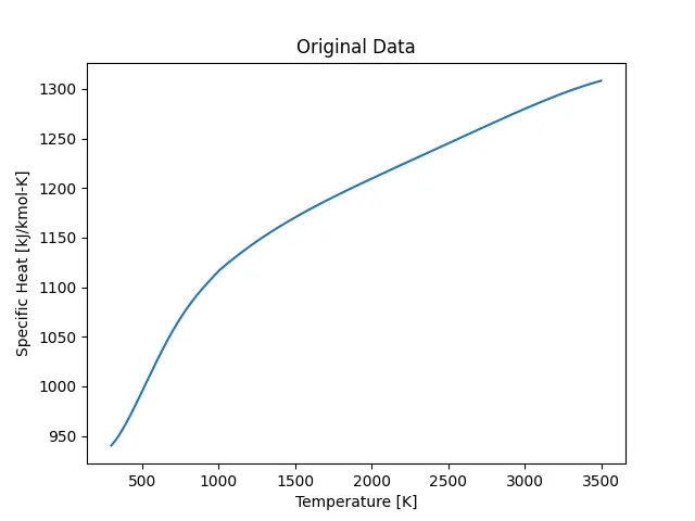
Figure 1: Original Data
The Figure 1 shows the graph plot between the values found in the file 'data'. This is the actual values of specific heat with respect to the temperature. The curves formed by Linear, Quadratic and Cubic polynomial fit will be compared to this graph to understand the accuracy or the best fit of the respective curve fits.
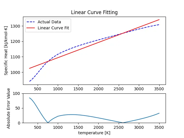
Figure 2: Linear Curve fit and its error curve
Figure 2 represents the Linear curve fit along with raw data. The error curve below represents the deviation of specific heat value formed by the linear curve fit from the original value at each value of temperature. Similarly, the Figure 3 shows the quadratic and cubic curve fits alon with the raw data and its corresponding error curves. This curve seems to fit more properly than the linear curve fit.
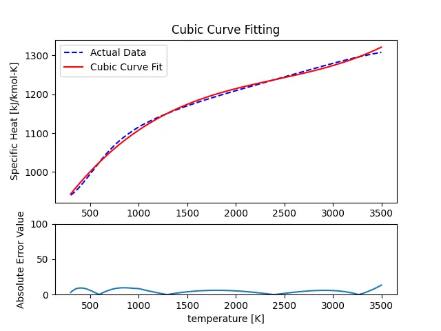
Figure 3: Cubic Curve fit and its error curve
Figure 4 depicts the graph plotted for comparison of each linear and cubic fit curves with respect to the original values. From the graph, it is clear that the cubic fit curve has more accurate value than the linear fit curve. To understand more, the error curve gives more idea where it represents the absolute value of error for the two curves at each temperature points. It is observed that the cubic curve fit has comparatively lesser error value than other followed by quadratic and linear. The maximum value of error found for linear curve fit is 84.4621 units while for cubic curve fit, the maximum error value is only 13.4401 units, which is a great reduction
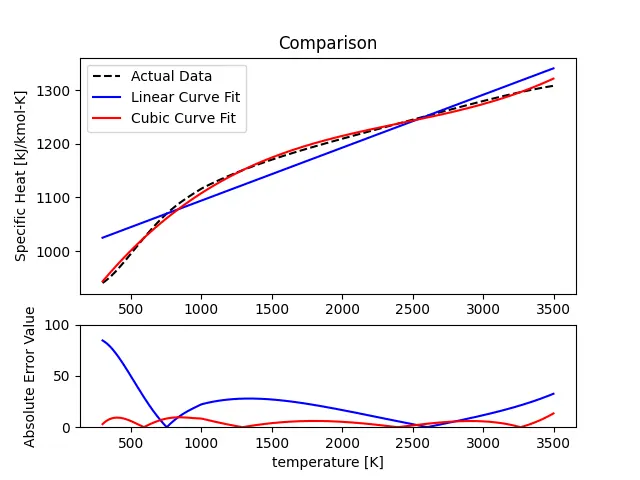
Figure 4: Comparison of Fit Curves
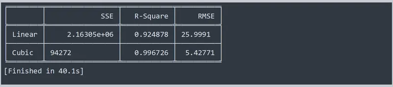
Figure 5: SSE, R-Square and RMSE value of linear and cubic curves.
Figure 5 represents the SSE, R-square and RMSE values for the linear and cubic curve fit. These values are used to find the best fit, that is, goodness of the fit or how well the equation is representing the datapoints. If the R-square is greater than 0.95, the fit is assumed to be good. Here, the cubic curve fit has R-square value greater than 0.95 which means that the linear curve fit here is not good.
Further Questions
- How to make a curve fit perfectly?
The curve that gives zero error between data y and the fit f(x) is the perfect fit. If the curve fit perfectly, then the R-square of the curve will equals one. Also, for perfect fit curve, the SSE quantity will be zero. The curve fit should match with the original data without showing the error in the command window. In order for setting the curve perfectly, we can eliminate the error by using the center and scaling code that is by elimination of error. - How to get the best fit? Note: Best fit and perfect fit are two completely different phenomena.
Consider the general form for a polynomial of order `j`
`f(x)=a_0+a_1x+a_2x^2+a_3x^3+...+a_jx^j =a_0+sum_(k=0)^ja_kx^k`
Let this be the equation for the curve fit. The curve that gives minimum error between data `y` and the fit `f(x)` is the best fit.
The best fit can be obtained by increasing the order of the polynomial and also by splitting the curves into multiple range and then plotting for each range set.
There are different methods to understand the goodness of the curve fit, namely The sum of squares due to error (SSE), R-square, Adjusted R-square and Root mean squared error (RMSE). From these quantities, we can evaluate the best fit of the curve. - What could be done to improve the cubic fit?
For improving the cubic fit, the splitwise method can be used where the data set in divided into multiple range. More the division, more will be the improvement to the curve.
Conclusion
The PYTHON program to fit a linear and cubic polynomial for the Cp data has been created successfully and has been plotted along with the raw data. The parameters such as SSE, R-square, Adjusted R-square and RMSE to measure the fitness characteristics of the curves has been understood and found.
References
[1]https://en.wikipedia.org/wiki/Curve_fitting
[2]https://skill-lync.com/projects/Curve-Fitting-and-criterion-to-choose-best-fit-41860
[3]https://ncss-wpengine.netdna-ssl.com/wp-content/themes/ncss/pdf/Procedures/NCSS/Introduction_to_Curve_Fitting.pdf
[4]https://www.iiserpune.ac.in/~bhasbapat/phy221_files/curvefitting.pdf
[5]https://statisticsbyjim.com/regression/curve-fitting-linear-nonlinear-regression/
[6] https://www.geeksforgeeks.org/python-statistics-mean-function/
[7] https://www.w3schools.com/python/matplotlib_subplots.asp