Simulation of Damped Harmonic Motion of a Simple Pendulum Using Matlab

AIM:

To write a program that solves the ODE representing the equation of motion of a simple pendulum with damping and to produce the simulation of motion for this damped oscillation.

OBJECTIVE:

1. To write the neccessary code to solve the 2nd order ODE of damped harmonic motion using MATLAB.
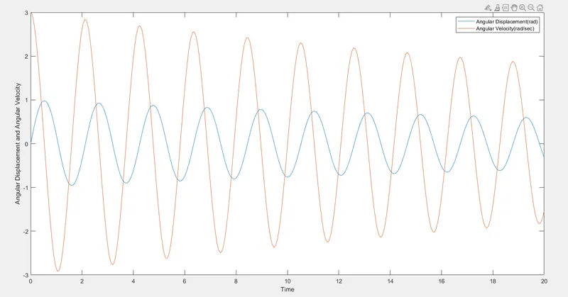
2. To plot the angular displacement and angular velocity variation with respect to time.
3. To create an animation to simulate this motion.

THEORY:

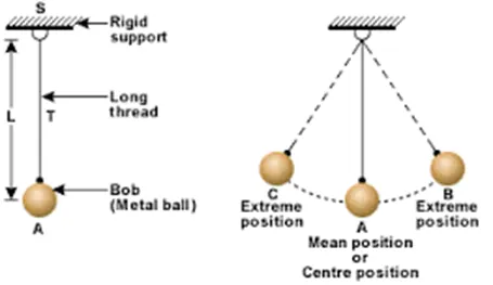
In Engineering, ODE is used to describe the transient behavior of a system. A simple example is a pendulum.

The way the pendulum moves depends on the Newtons second law. When this law is written down, we get a second order Ordinary Differential Equation that describes the position of the "bob" with respect to time.

Similarly, there are hundreds of ODEs that describe key phenomena and if you have the ability to solve these equations then you will be able to simulate any of theses systems.

When the motion of an oscillator reduces due to an external force, the oscillator and its motion are damped. These periodic motions of gradually decreasing amplitude are damped simple harmonic motion. An example of a damped simple harmonic motion is a simple pendulum.

In the damped simple harmonic motion, the energy of the oscillator dissipates continuously. But for a small damping, the oscillations remain approximately periodic. The forces which dissipate the energy are generally frictional forces.

The general ODE equation we are trying to solve here is this:

`(del^2theta)/(delt^2)+ b/m*(deltheta)/(delt)+ g/L *sintheta = 0`

Where,

`theta` = Angular Displcement in radians

b = Damping Coefficient

m = Mass of the pendulum in kg

g = Acceleration due to gravity in `m/s^2`

L = Length of the pendulum in meter (m)

SIMPLIFYING THE 2ND ORDER ODE TO SOLVE IT USING MATLAB:

Assume, `theta = theta1`

`(deltheta)/(delt) = (deltheta1)/(delt) = theta2`

`(deltheta1^2)/(delt^2) = (deltheta2)/(delt)`

Equation Becomes:

`(deltheta2)/(delt) + b/m * theta2 + g/L * sintheta1 = 0`

2nd order ODE reduces to two 1st order ODE:

`(deltheta1)/(delt) = theta2`

`(deltheta2)/(delt) = (-b)/m * theta2 - g/L * sintheta1`

MAIN CODE OF THE PROGRAM:

clear all
close all
clc

g=9.81;           % Acceleration  due to gravity in m/s2
L=1;              % length of the pendulum in meter
b=0.05;           % damping coefficient
m=1;              % mass of the pendulum in kg
t = [0 20];       % time period of the harmonic motion/limits
theta0 = [0 3];   % initial and boundary conditions of angular displacement

[t theta]= ode45(@(t,theta) odefun_second_order_pendulum(t,theta,g,L,b,m),t,theta0); % solving the 2nd order ODE using the function odefun_second_order_pendulum

figure(1)

plot(t,theta(:,1),t,theta(:,2)) % Plotting the angular dispcement and angular velocity vs time graph of the specified motion
ylabel('Angular Displacement and Angular Velocity')
xlabel('Time')
legend('Angular Displacement(rad)','Angular Velocity(rad/sec)')

% Code for animation of the pendulum 

ct=1; % Initialising loop counter
for i=1:length(t)
    figure(2)
    plot([-1 1],[0 0]); % plotting the wall where the pendulum is fixed
    axis([-1.5 1.5 -1.5 1]); % defining the limits of values in the x and y axis
    hold on
    plot(L*sin(theta(i,1)),-L*cos(theta(i,1)),'o','markersize',20,'markerfacecolor','w'); % plotting the bobof the pendulum
    hold on
    plot([0,L*sin(theta(i,1))],[0,-L*cos(theta(i,1))],'b'); % Plotting the string of the pendulum
    hold off
    M(ct)=getframe(gcf); % stiching all frame in M array to create an animation
    ct=ct+1;
end

movie(M)
videofile = VideoWriter('Damped_Pendulum.avi', 'Uncompressed AVI');

open(videofile)
writeVideo(videofile,M)
close(videofile)

FUNCTION CODE:

function [thetadot] = odefun_second_order_pendulum(t,theta,g,L,b,m)
thetadot = zeros(2,1);
thetadot(1)= theta(2);
thetadot(2)= ((-b/m)*theta(2)) - ((g/L)*sin(theta(1)));
end

OBSERVATIONS/OUTPUT:

Variation of Angular Displacement and Angular Velocity with respect to time

SIMULATION OF THE DAMPED HARMONIC MOTION OF PENDULUM :

CONCLUSION:

• The neccessary MATLAB code to solve the 2nd order ODE of damped harmonic motion was constructed.
• Plotted the angular displacement and angular velocity variation with respect to time.
• The animation of the simulation of the damped harmonic motion of pendulum is constructed.

Link To Code: https://drive.google.com/file/d/1zxyl6aUGeNIdXoBsvVLIfGm78q_A4_W4/view?usp=sharing

https://drive.google.com/file/d/14GY4ekT2m4DOOKBU667_Jron4LZpkf-L/view?usp=sharing