Second Order ODE to get the position of the pendulum as a function of time

AIM:

To solve the ODE equation represents the equation of motion of a simple pendulum with damping to get the position of the pendulum as a function of time.

Fomulae used:

`(d^2theta)/dt^2 + b/m*(d theta)/dt+g/l*sintheta=0`

# where (d^2theta/dt^2) represents the second order ODE.

# b = damping force

# m = mass

# g = gravity

# l = length

Project Objective:

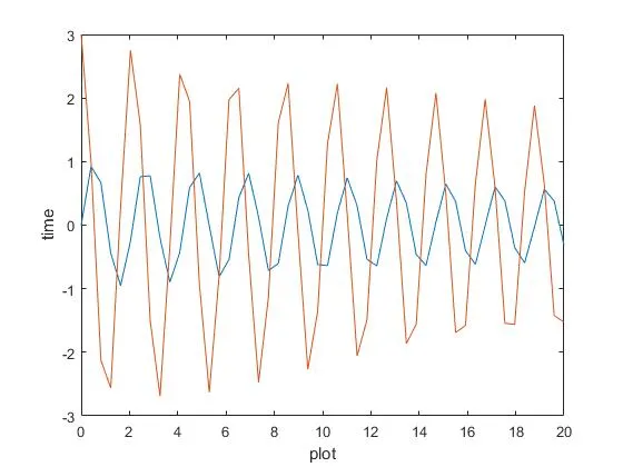
# The main objective of the project is to solve the second order ODE for a simple pendulum with damping. The plotting for graph to the simple pendulum with respect to time and creating a movie animation to show the moving of ball in simple pendulum is executed in the project.

# The work flow is started from solving the second order ODE function and flow continues to defining the inputs given on problem are considered where the intial conditions for displacement and velocity is taken for writing the code. Integrating the ODE function to obtain the solution and time span is followed.

Program Description:

The programming language used here is HTML

clear all
close all
clc

b = 0.05;
g = 9.81;
l = 1;
m = 1;

% initial condition
theta_0 = [0;3];

% time points
t_span = linspace(0,20,300);

% solve ODE
[t, results] = ode45(@(t,theta)ode_func(t,theta,b,g,l,m),t_span,theta_0);

plot(t, results(:,1))
hold on
plot(t, results(:,2))
xlabel('plot')
ylabel('time')

fig = 1;

for i = 1:length(t)
    
%initial position of the pendulum
x0 = 0;
y0 = 0;

%final position
x1 = l*sin(results(i,1));
y1 = -1*cos(results(i,1));

%plotting
figure(2)
%baseline
plot([-1,1],[0,0],'linewidth',5,'color','b')
hold on

%pendulum line
plot([x0,x1],[y0,y1],'linewidth',3,'color','r')
hold on

%pendulum ball
plot(x1,y1,'marker','o','markersize',25,'markerfacecolor','y')
grid on

axis([-2 2 -2 1]);
pause(0.01);
hold off;
M(fig) = getframe(gcf);
fig = fig+1;

end

movie(M)
videofile = VideoWriter('second_ode_solving.avi','uncompressed AVI')
open(videofile)
writeVideo(videofile,M)
close(videofile)

ode function is created by writing this script below

function [dtheta_dt] = ode_func(t,theta,b,g,l,m)
theta1 = theta(1)
theta2 = theta(2)
dtheta1_dt = theta2;
dtheta2_dt = -(b/m)*theta2 - (g/l)*sin(theta1);
dtheta_dt = [dtheta1_dt; dtheta2_dt];

end

# The inputs for the code is written. for the values of b, g, l, m.

# There are two first order ode one is for displacement and other one is for velocity.

# theta_0=[0;3]; where the initial value for displacement is zero and the initial value for velocity is 3 is written.

# To solve the first order ode we need to initiliaze conditions for displacement

# t_span = (0, 20, 300) , where t_span is called time array which (0-20) is the time specified in the given problem and 300 is the interval time between (0-20).

# [t=results] = ode45(@(t,theta)ode_func(t,theta,b,g,l,m0,t_span,theta_0; where ode45 is an inbuilt solver in matlab and its annonoumous function in matlab. (t, theta) are dependent variable and independent variable of the ode system. Our ode is the function of (t,theta). the the ode_func is defined.

# ode_func is a seperate matlab program that is written along with this script writing to acces the ode_func.

# To create the image to represent the position of pendulum with respect to time the plotting command is used with respect to the results by calling for loop command.

# Hold on command is used to keep the current plot while adding new element. label command is used to represent the axis in the plot diagram.

# fig = 1 generates the figure in window 1

# Initial condition & final condition for the pendulum is defined.

# The condition for baseline is given with axis points, where linewidth is used to define the width of line. and color command is used for giving the line colour.

# hold on is used again for adding new elements.

# The condition for pendulum line is given with axis points, where linewidth is used to define the width of line. and color command is used for giving the line colour and hold on is used.

# The condition for pendulum ball is given with axis points, where o represent the ball shape, marker is the command used to create the circle here and marker size is used to specify the size of ball. Markerfacecolor command is used to give the color.

# axis is defined for creating the animation where (-2 2 2 0) is (x0 xfinal y0 yfinal)

# M(ct) = getframe(gcf) is called to create a movie the command is called.

# end command is used due to for loop is used.

# Videofile = VideoWriter('second_ode_solving.avi', 'uncompressed AVI') which second_ode_solving is the name used for saving the code that is to be used for creating a movie.

Graph:

Animation:

Mistakes done:

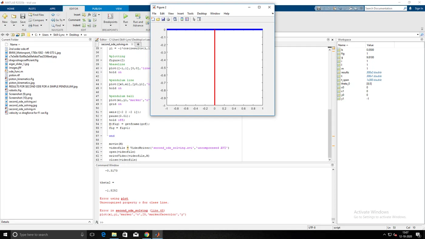
plot(x1,y1,'marker','o',25,'markerfacecolor','y')- the command line has error in execution where marker size is missed in writing the code.

# the corrected one is plot(x1,y1,'marker','o','markersize',25,'markerfacecolor','y')

Mistakes overcome:

The mistake overcome is done by taking the notes.

Conclusion:

The graph and animation for the equation simple pendulum with respective to time is plotted and animated.