Matlab program for NASA thermodynamic data file parsing

AIM:

To write a function for the thermodynamic data file of NASA that extracts the 14 coefficients and calculates the enthalpy, entropy, and specific heats for all the species in the data file.

OBJECTIVE:

# Low temperature and high-temperature ranges are separated for the 14 coefficients.

# Local temperature ranges is taken not the global temperature ranges.

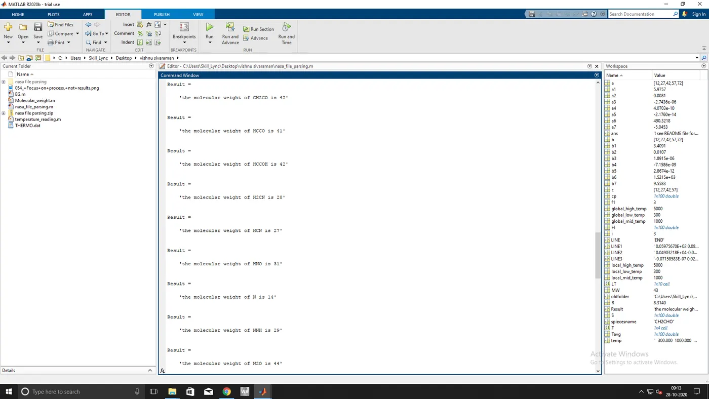
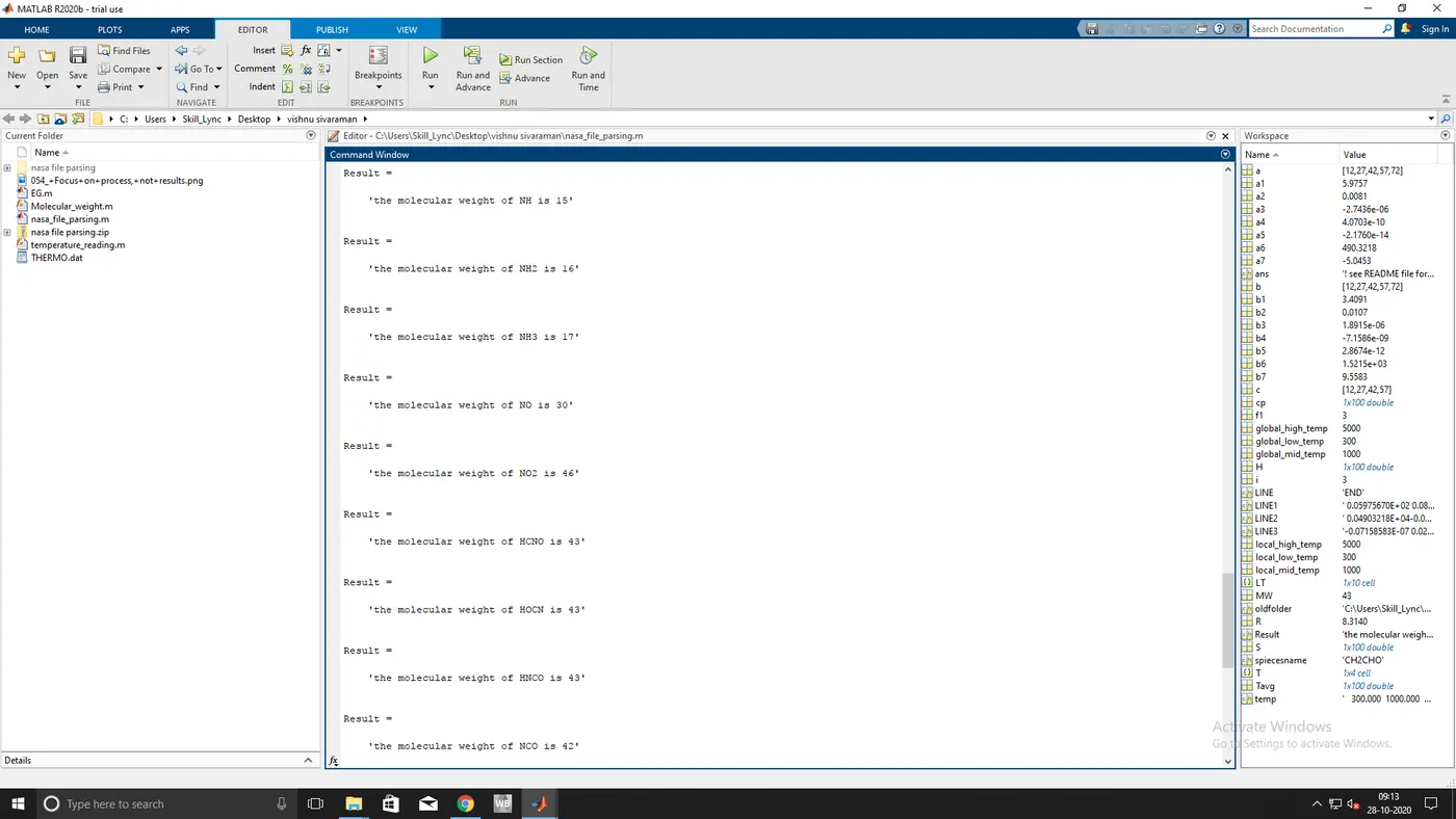
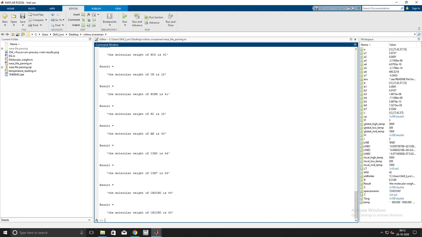
# Molecular weight of each species to be calculated and to be displayed in the command window.

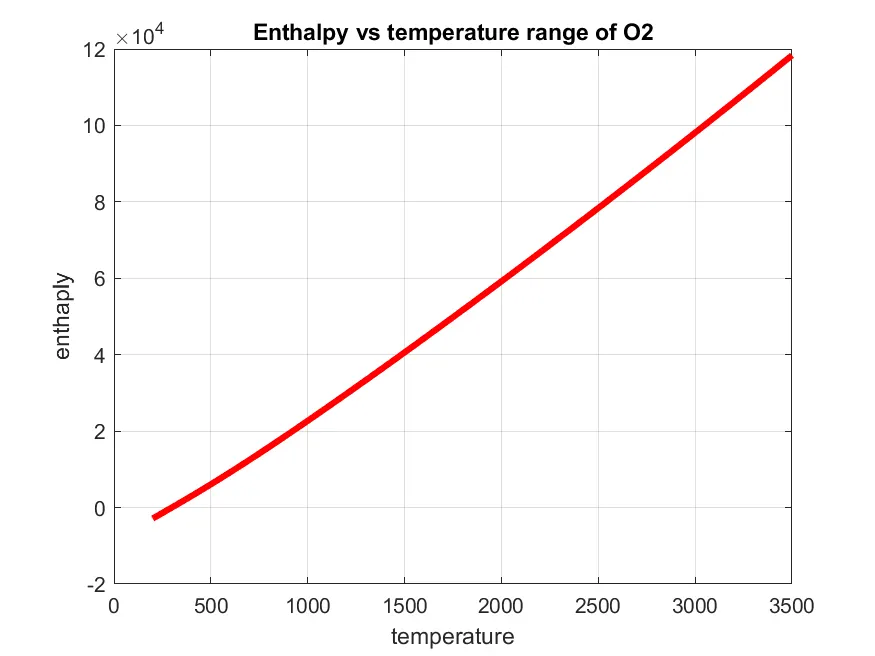
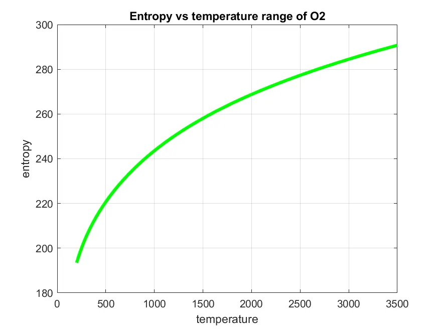
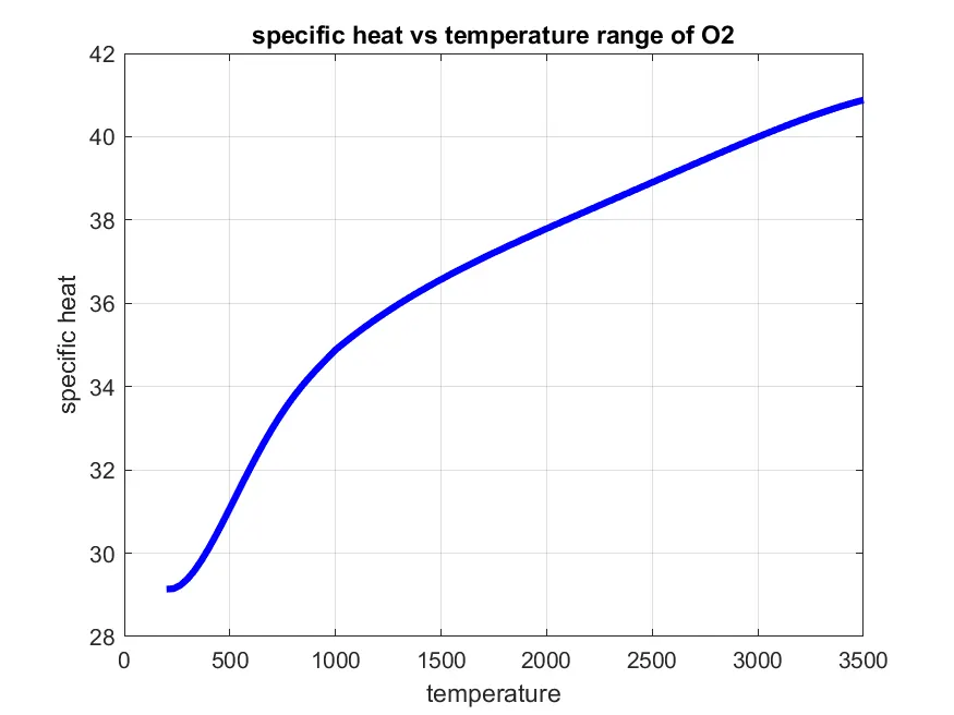
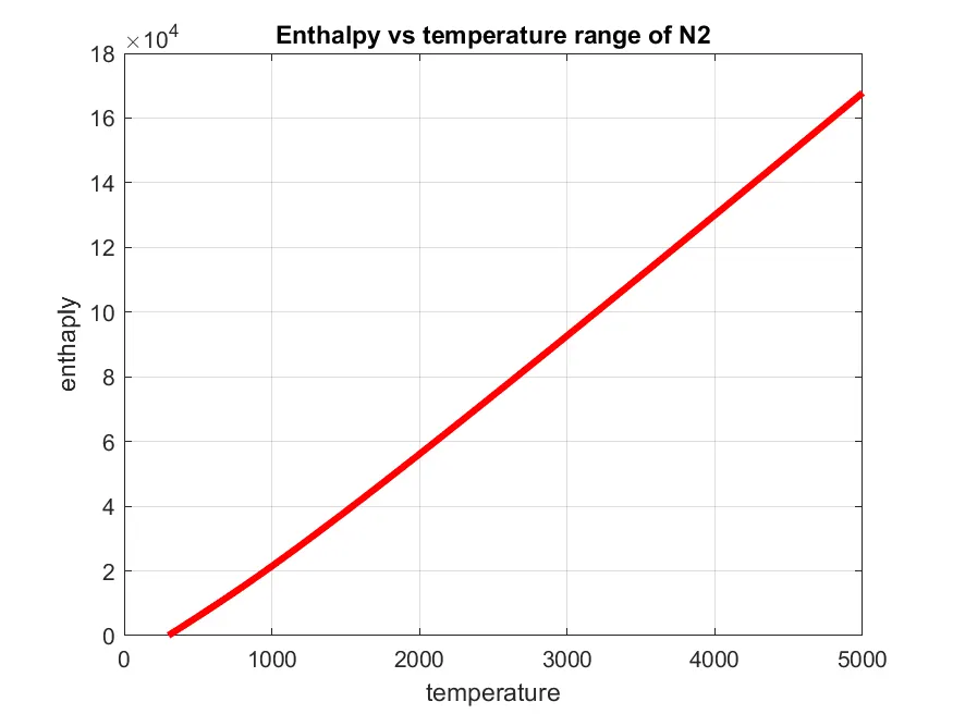
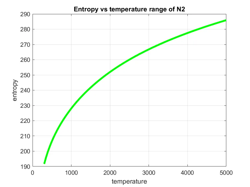
# cp, enthalpy, entropy, low temperature, high temperature specific for each species will be plotted.

# plots are saved in a separate folder with proper species name.

PROCEDURE:

Data parsing is a method where one string of data gets converted into a different type of data. So let’s say you receive your data in raw HTML, a parser will take the said HTML and transform it into a more readable data format that can be easily read and understood.

Here R is the universal gas constant and T is temperature.

clear all
close all
clc
%reading thrmo data file
f1 = fopen('THERMO.dat','r')
fgetl(f1);
% Defining gas constant
R = 8.314;

Where the program is written by calling the data file to extract the values from the dat.file, data is loaded by calling the fopen. fgetl is used for skipping the header. The f1 under fgetl is the place of the file under fgetl. The gas constant is defined by providing the values.

% Extracting global temperature data
temp = fgetl(f1);
T = strsplit(temp);
global_low_temp = str2num(T{2});
global_mid_temp = str2num(T{3});
global_high_temp = str2num(T{4});

The global temperature data is extracted and strsplit is used for the elements of delimiter. The global temperature is in the second line so we are using fgetl second time so it will read the temperatures as strings. By using str2num we can convert it into a number so we can get the global low, mid, high-temperature ranges.

%skipping the comments 
for i= 1:3
fgetl(f1);
end
while true
LINE=fgetl(f1)
if LINE=="END"
break
end

Skipping the comments where for loop is called. Hence the loop will run for three lines though skipping them. In order to make code shorter, we will be finding the species values by using while loop where break the loop 'END' is used at the end of the file. We can also use for loop but while using for loop the number of times the loop needs to be run should be known. so while loop is used in the code.

%Reading all the spieces
spiecesname = (strtok(LINE));
LT = strsplit(LINE)

strtok ignores whitespaces and captures the first letter or word. After that we will be using strsplit command to split the whitespaces

% Reading global temperature spieces
local_low_temp = str2num(LT{end-3});
local_mid_temp = str2num(LT{end-1});
local_high_temp = str2num(LT{end-2});

str2num is used to capture the local temperature for local low, mid, high-temperature range.

% Reading LINE1 of temperature values
LINE1 = fgetl(f1)
a = strfind(LINE1,'E');

The average temperature will be in the range local to high temperature. In order to find out the position coefficients, we need to find out the position of 'E' by using strfind command.

%Converting string values to numbers
a1 = str2num(LINE1(1:a(1)+3));
a2 = str2num(LINE1(a(1)+4:a(2)+3));
a3 = str2num(LINE1(a(2)+4:a(3)+3));
a4 = str2num(LINE1(a(3)+4:a(4)+3));
a5 = str2num(LINE1(a(4)+4:a(5)+3));
% Reading LINE2 of temperature values
LINE2=fgetl(f1)
b=strfind(LINE2,'E')
%Converting string values to numbers
a6 = str2num(LINE2(1:b(1)+3));
a7 = str2num(LINE2(b(1)+4:b(2)+3));
b1 = str2num(LINE2(b(2)+4:b(3)+3));
b2 = str2num(LINE2(b(3)+4:b(4)+3));
b3 = str2num(LINE2(b(4)+4:b(5)+3));
% Reading LINE3 of temperature values
LINE3 = fgetl(f1)
c = strfind(LINE3,'E');
% converting string values to numbers
b4 = str2num(LINE3(1:c(1)+3));
b5 = str2num(LINE3(c(1)+4:c(2)+3));
b6 = str2num(LINE3(c(2)+4:c(3)+3));
b7 = str2num(LINE3(c(3)+4:c(4)+3));

From a1 to a7 are high-temperature range and from b1 to b7 are low-temperature coefficients and with the position of 'E' we will be calculating the coefficients. By using str2num the string is converted into a number.

The formula used to find specific heat, enthalpy, entropy:

`(Cp)/R=a1+a2*T+a3*T^2+a4*T^3+a5*t^4`

`H/(RT)=a1+a2*T/2+a3*T^2/3+a4*T^3/4+a5*T^4/5+(a6)/t`

`S/R=a1*logT+a2*T+a3*T^2/2+a4*T^3/3+a5*T^4/4+a7`

Formula is written as a function to make the code easier

function[cp,H,S] = temperature_reading(a1,a2,a3,a4,a5,a6,a7,b1,b2,b3,b4,b5,b6,b7,R,Tavg,local_mid_temp)
for i = 1:length(Tavg)
if Tavg(i) > local_mid_temp
cp(i)= R*(a1+a2*Tavg(i)+a3*(Tavg(i)^2)+a4*(Tavg(i)^3)+a5*Tavg(i)^4);
H(i)= R*Tavg(i)*(a1+a2*(Tavg(i)/2)+a3*(Tavg(i)^2/3)+a4*(Tavg(i)^3/4)+a5*(Tavg(i)^4/5)+a6/Tavg(i));
S(i)= R*(a1*log(Tavg(i))+a2*Tavg(i)+a3*(Tavg(i)^2/2)+a4*(Tavg(i)^3/3)+a5*(Tavg(i)^4/4)+a7);
else
cp(i)= R*(b1+b2*Tavg(i)+b3*(Tavg(i)^2)+b4*(Tavg(i)^3)+b5*Tavg(i)^4);
H(i)= R*Tavg(i)*(b1+b2*(Tavg(i)/2)+b3*(Tavg(i)^2/3)+b4*(Tavg(i)^3/4)+b5*(Tavg(i)^4/5)+b6/Tavg(i));
S(i)= R*(b1*log(Tavg(i))+b2*Tavg(i)+b3*(Tavg(i)^2/2)+b4*(Tavg(i)^3/3)+b5*(Tavg(i)^4/4)+b7);
end
end
end

Here by writing this above function here we will be calculating enthapy, entropy, specific heat by using a single function. for loop is used so we can calculate the value of T_avg. So the T_avg will range from local low to local high temperature range. b1 to b7 are local coefficient for local low temperature range anf a1 to a7 are the local coefficient for local high temperature range. if condition is used here to find the local low coefficients will be used to calculate the values of high coefficients.

% calculating Specfic heat, enthalpy, entropy
[cp,H,S] = temperature_reading(a1,a2,a3,a4,a5,a6,a7,b1,b2,b3,b4,b5,b6,b7,R,Tavg,local_mid_temp);

To call the function to calculate the enthalpy, entropy, specific heat is written above.

mkdir('C:UsersSkill_LyncDesktopvishnu sivaramannasa file parsing',spiecesname);

mkdir will create the folder in the given directory and given element name as the folder which stores the graph of each species for the enthalpy, entropy, specific heat for the temperature.

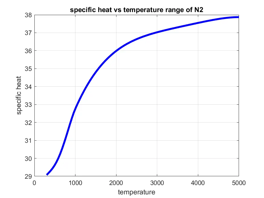
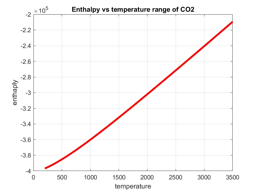
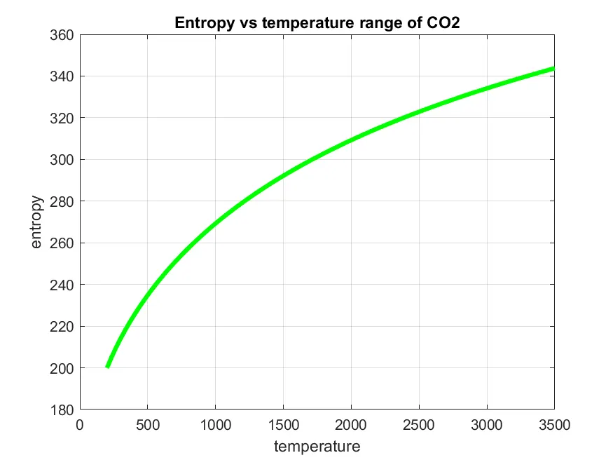
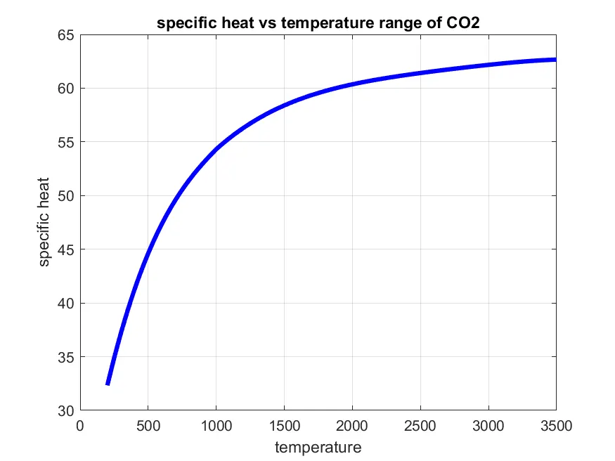
The next step is to plot all the elements of entropy, enthalpy, specific heat VS temperature range of all species.

figure(1)
plot(Tavg,cp,'linewidth',3,'color','b')
title(sprintf('specific heat vs temperature range of %s',spiecesname))
xlabel('temperature')
ylabel('specific heat')
grid on
figure(2)
plot(Tavg,H,'linewidth',3,'color','r')
title(sprintf('Enthalpy vs temperature range of %s',spiecesname))
xlabel('temperature')
ylabel('enthaply')
grid on
figure(3)
plot(Tavg,S,'linewidth',3,'color','g')
title(sprintf('Entropy vs temperature range of %s',spiecesname))
xlabel('temperature')
ylabel('entropy')
grid on

sprintf is used for the title to change the name for each species while generating the plot in each loop. The other other commands are usual that we used before to plot the graph.

cd(['C:UsersSkill_LyncDesktopvishnu sivaramannasa file parsing',spiecesname]);
saveas (1,'Tavg vs Specific_heat.png')
saveas (2,'Tavg vs Enthalpy.png')
saveas (3,'Tavg vs Entropy.png')
oldfolder = cd('C:UsersSkill_LyncDesktopvishnu sivaraman');

To save the graph we need to give a new directory where we have created the folder with species name so we have used the cd command here to save the figure1, figure2, and figure3. The old folder command is used to save the files in the given old directory will change when the graph is plotted.

A function is written to find the molecular weight for all species

function[MW] = Molecular_weight(speciesname);
Atoms = ['O','H','C','N','A'];
Atomic_number = [16 1 12 14 40];
MW=0;
for i =1:length(speciesname);
for j = 1:length(Atoms);
if strcmpi(speciesname(i),Atoms(j));
MW=MW+Atomic_number(j);
position=j;
end
end
n = str2num(speciesname(i));
if n>1;
MW = MW+Atomic_number(position)*(n-1);
end
end

Molecule and molecular mass have to be specified and atoms and atomic numbers have to be provided. Here the atoms are individual which are given in the data. Molecular weight is taken as zero before starting the loop.

Nested for loop is used to find the molecular weight where the first loop will run for the species and the second loop will run for the length of atoms. The position command will capture the location of the letter in the atom array.

full script for NASA file parsing

clear all
close all
clc
%reading thrmo data file
f1 = fopen('THERMO.dat','r')
fgetl(f1);
% Defining gas constant
R = 8.314;

% Extracting global temperature data
temp = fgetl(f1);
T = strsplit(temp);
global_low_temp = str2num(T{2});
global_mid_temp = str2num(T{3});
global_high_temp = str2num(T{4});
%skipping the comments 
for i= 1:3
fgetl(f1);
end
while true
LINE=fgetl(f1)
if LINE=="END"
break
end

%Reading all the spieces
spiecesname = (strtok(LINE));
LT = strsplit(LINE)

% Reading global temperature spieces
local_low_temp = str2num(LT{end-3});
local_mid_temp = str2num(LT{end-1});
local_high_temp = str2num(LT{end-2});

% Reading LINE1 of temperature values
LINE1 = fgetl(f1)
a = strfind(LINE1,'E');
%Converting string values to numbers
a1 = str2num(LINE1(1:a(1)+3));
a2 = str2num(LINE1(a(1)+4:a(2)+3));
a3 = str2num(LINE1(a(2)+4:a(3)+3));
a4 = str2num(LINE1(a(3)+4:a(4)+3));
a5 = str2num(LINE1(a(4)+4:a(5)+3));

% Reading LINE2 of temperature values
LINE2=fgetl(f1)
b=strfind(LINE2,'E')
%Converting string values to numbers
a6 = str2num(LINE2(1:b(1)+3));
a7 = str2num(LINE2(b(1)+4:b(2)+3));
b1 = str2num(LINE2(b(2)+4:b(3)+3));
b2 = str2num(LINE2(b(3)+4:b(4)+3));
b3 = str2num(LINE2(b(4)+4:b(5)+3));

% Reading LINE3 of temperature values
LINE3 = fgetl(f1)
c = strfind(LINE3,'E');
% converting string values to numbers
b4 = str2num(LINE3(1:c(1)+3));
b5 = str2num(LINE3(c(1)+4:c(2)+3));
b6 = str2num(LINE3(c(2)+4:c(3)+3));
b7 = str2num(LINE3(c(3)+4:c(4)+3));

% Defining temperature range for calculations
Tavg = linspace(local_low_temp,local_high_temp,100);
% calculating Specfic heat, enthalpy, entropy
[cp,H,S] = temperature_reading(a1,a2,a3,a4,a5,a6,a7,b1,b2,b3,b4,b5,b6,b7,R,Tavg,local_mid_temp);

%plotting graph for specific_heat, enthalpy and entropy
%creating a separate folder and files for molecular data for spieces 
mkdir('C:UsersSkill_LyncDesktopvishnu sivaramannasa file parsing',spiecesname);
figure(1)
plot(Tavg,cp,'linewidth',3,'color','b')
title(sprintf('specific heat vs temperature range of %s',spiecesname))
xlabel('temperature')
ylabel('specific heat')
grid on

figure(2)
plot(Tavg,H,'linewidth',3,'color','r')
title(sprintf('Enthalpy vs temperature range of %s',spiecesname))
xlabel('temperature')
ylabel('enthaply')
grid on

figure(3)
plot(Tavg,S,'linewidth',3,'color','g')
title(sprintf('Entropy vs temperature range of %s',spiecesname))
xlabel('temperature')
ylabel('entropy')
grid on
cd(['C:UsersSkill_LyncDesktopvishnu sivaramannasa file parsing',spiecesname]);
saveas (1,'Tavg vs Specific_heat.png')
saveas (2,'Tavg vs Enthalpy.png')
saveas (3,'Tavg vs Entropy.png')
oldfolder = cd('C:UsersSkill_LyncDesktopvishnu sivaraman');
MW = Molecular_weight(spiecesname); 
Result = sprintf('the molecular weight of %s is %d',spiecesname,MW)
end

plots for all species are saved in the given directory

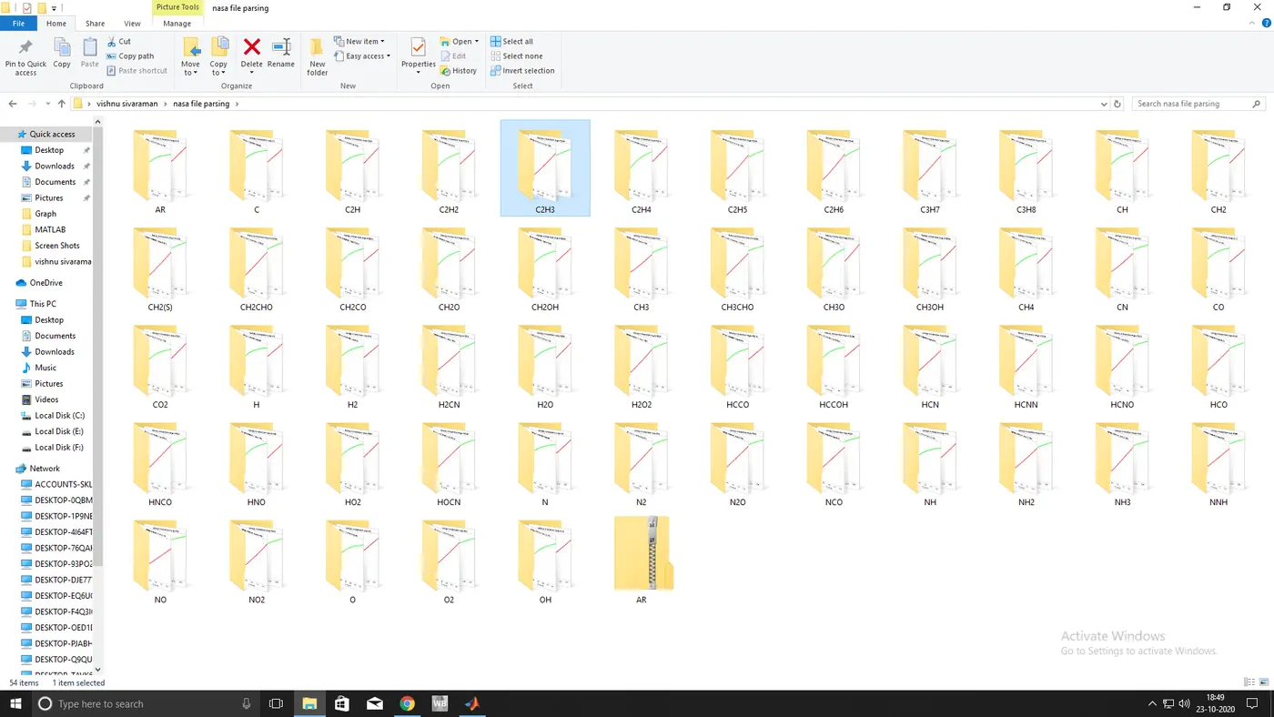
And link to access these files is given below:

https://drive.google.com/file/d/1z6xuQgHSXV-SSe4YDPIqX6L4aZ02Cg93/view?usp=sharing

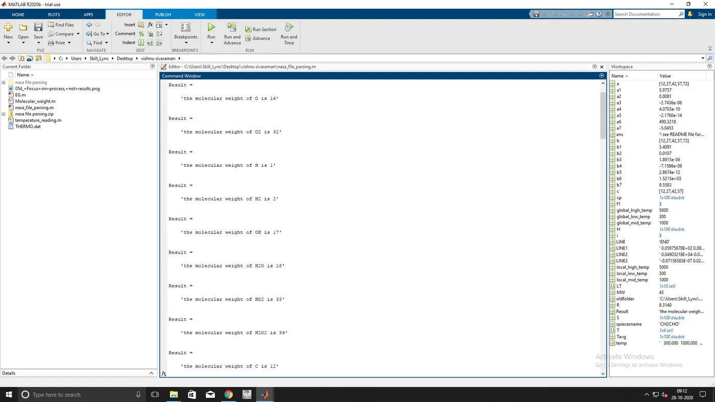
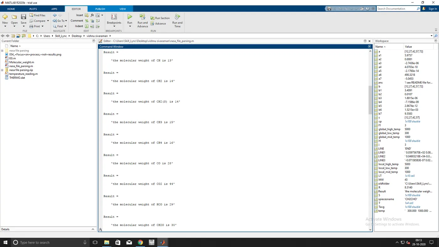
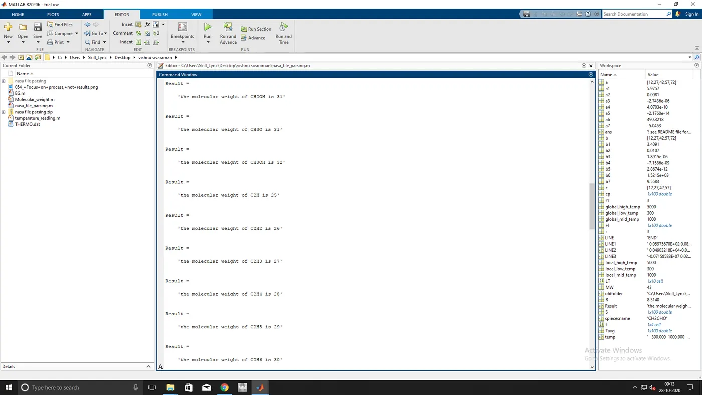
Command window results are shown below:

plots for O2:

plots for N2:

plots for CO2:

Conclusion:

Where the script for NASA thermodynamic data file parsing to extracts the coefficients with respect to the temperature graphs are plotted and the molecular weight is found.