matlab program for a curve fit for splitwise polynomial
AIM:
To write a code to fit a linear and cubic polynomial for the given cp data and temperature
Project Objective:
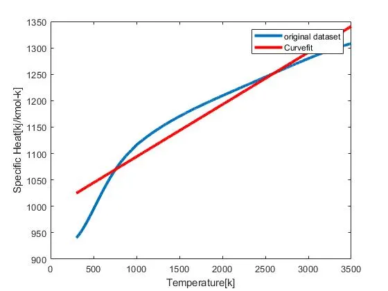
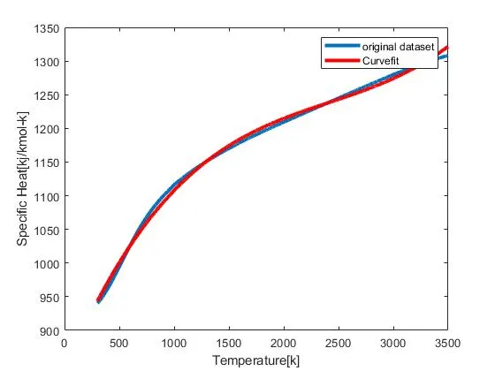
Plotting the linear and cubic fit curves along with raw data points, the title label, axis and legends are to shown in graph. The main objective of this curve fit code is to set the original data line with curve fit created. The polynomial order is used to fit the curve perfectly with the original data set. fitness characteristics for both the curve should be measured.
Formula:
`SSE = sum_i^n = Err(i)^2`
`R^2 = (SSR)/(SSE)` where R^2 = 0 to 1 which is 0 for worst possible fit and 1 for best possible fit
SSR = Sum of square of the regression, which is basically the square of the difference between the value of the fitting function at a given point
SSE = Sum of squared errors
`SSR1 =((pred_cp - (m))^2)` where predicted overall cp - mean is taken into account for calculation.
`SST = SSR + SSE` Sum of squred error and regression is added to form SST
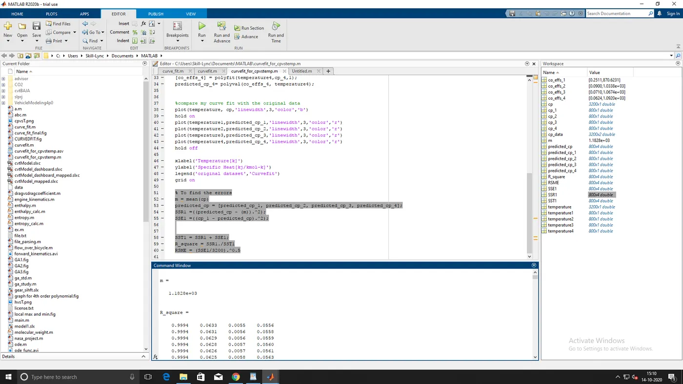
The value of R^2 greater than 0.95 is assumed to be good fit.
`RSME = root _((SSE)/n)`
Code explanation for linear polynomial:
clear all
close all
clc

%preparing the data
cp_data = load('data');

temperature = cp_data(:,1);
cp = cp_data(:,2);

%plot

%curve fit
%cp = a*T+b
co_effs = polyfit(temperature,cp,1);
predicted_cp = polyval(co_effs, temperature);

%compare my curve fit with the original data
plot(temperature, cp,'linewidth',3)
hold on
plot(temperature,predicted_cp,'linewidth',3,'color','r')
xlabel('Temperature[k]')
ylabel('Specific Heat[kj/kmol-k]')
legend('original dataset','Curvefit')
# The above code is written for linear polynomial to the given cp_data and temperature value.
# cp_data = load('data'); is the command used to call the data file into the code.
# temperature = cp_data(:,1); where the temperature is equal for the cp_data of the first column.
# cp = cp_data(:,2); the temperature is equal for the cp_data of the second column .
# The plotting of coordinates for linear polynomial codes are explained with its x and y axis.
# %cp = a*T+b - formula for the first order polynomial.
# co_effs = polyfit(temperature,cp,1); polyfit creates the coefficient of polynomial which is used to set the curve data, and (temp,cp,1) refers to x-axis, y-axis & order for polynomial.
# predicted_cp = polyval(co_effs, temperature); polyval is the polynomial value where for co_effs the polynomial coefficients is required first and temp refers the 'x' data set.
# plot(temperature, cp,'linewidth',3) the command is used to plot the original data set. where the cp is called on y-axis to represent original value.
# hold on is used adding the new set of values.
# plot(temperature,predicted_cp,'linewidth',3,'color','r') the command is used to plot the curvefit data set. where the predicted_cp is called on y-axis to represent curvefit value.
# The commands are used to compare the datas between original and curvefit to plot a graph.
# x-label command is used to represent x-axis.
# y-label command is used to represent y-axis.
# legend command is used for showing the scale in graph.
Plot diagram for linear polynomial:
Code explanation for cubic polynomial:
clear all
close all
clc

%preparing the data
cp_data = load('data');

temperature = cp_data(:,1);
cp = cp_data(:,2);

%plot

%curve fit
%cp = a*T^3 + b*T^2 + C*T + d
co_effs = polyfit(temperature,cp,3);
predicted_cp = polyval(co_effs, temperature);

%compare my curve fit with the original data
plot(temperature, cp,'linewidth',3)
hold on
plot(temperature,predicted_cp,'linewidth',3,'color','r')
xlabel('Temperature[k]')
ylabel('Specific Heat[kj/kmol-k]')
legend('original dataset','Curvefit')
# The above code is written for cubic polynomial to the given cp_data and temperature value.
# cp_data = load('data'); is the command used to call the data file into the code.
# temperature = cp_data(:,1); where the temperature is equal for the cp_data of the first column.
# cp = cp_data(:,2); the temperature is equal for the cp_data of the second column .
# The plotting of coordinates for linear polynomial codes are explained with its x and y axis.
# %cp = a*T^3 + b*T^2 + C*T + d - formula for the cubic order polynomial.
# co_effs = polyfit(temperature,cp,3); polyfit creates the coefficient of polynomial which is used to set the curve data, and (temp,cp,3) refers to x-axis, y-axis & order for polynomial.
# predicted_cp = polyval(co_effs, temperature); polyval is the polynomial value where for co_effs the polynomial coefficients is required first and temp refers the 'x' data set.
# plot(temperature, cp,'linewidth',3) the command is used to plot the original data set. where the cp is called on y-axis to represent original value.
# hold on is used adding the new set of values.
# plot(temperature,predicted_cp,'linewidth',3,'color','r') the command is used to plot the curvefit data set. where the predicted_cp is called on y-axis to represent curvefit value.
# The commands are used to compare the datas between original and curvefit to plot a graph.
# x-label command is used to represent x-axis.
# y-label command is used to represent y-axis.
# legend command is used for showing the scale in graph.
Plot diagram for cubic polynomial:
Code explanation for splitwise method
clear all
close all
clc

%preparing the data
cp_data = load('data');
temperature = cp_data(:,1);
cp = cp_data(:,2);

temperature1 = cp_data(1:800,1);
cp_1 = cp_data(1:800,2);

temperature2 = cp_data(801:1600,1);
cp_2 = cp_data(801:1600,2);

temperature3 = cp_data(1601:2400,1);
cp_3 = cp_data(1601:2400,2);

temperature4 = cp_data(2401:3200,1);
cp_4 = cp_data(2401:3200,2);

%curve fit
%cp_1 = a*T + b
[co_effs_1] = polyfit(temperature1,cp_1,1);
predicted_cp_1 = polyval(co_effs_1, temperature1);

[co_effs_2] = polyfit(temperature2,cp_2,1);
predicted_cp_2 = polyval(co_effs_2, temperature2);

[co_effs_3] = polyfit(temperature3,cp_3,1);
predicted_cp_3= polyval(co_effs_3, temperature3);

[co_effs_4] = polyfit(temperature4,cp_4,1);
predicted_cp_4= polyval(co_effs_4, temperature4);


%compare my curve fit with the original data
plot(temperature, cp,'linewidth',3,'color','b')
hold on
plot(temperature1,predicted_cp_1,'linewidth',3,'color','r')
plot(temperature2,predicted_cp_2,'linewidth',3,'color','r')
plot(temperature3,predicted_cp_3,'linewidth',3,'color','r')
plot(temperature4,predicted_cp_4,'linewidth',3,'color','r')
hold off

xlabel('Temperature[k]')
ylabel('Specific Heat[kj/kmol-k]')
legend('original dataset','Curvefit')
grid on

% To find the errors
m = mean(cp)
predicted_cp = [predicted_cp_1, predicted_cp_2, predicted_cp_3, predicted_cp_4];
SSR1 =((predicted_cp - (m)).^2);
SSE1 =((cp_1 - predicted_cp).^2);


SST1 = SSR1 + SSE1;
R_square = SSR1./SST1
RSME = (SSE1/3200).^0.5
# The above code is written for cubic polynomial to the given cp_data and temperature value.
# cp_data = load('data'); is the command used to call the data file into the code.
# temperature = cp_data(:,1); where the temperature is equal for the cp_data of the first column.
# cp = cp_data(:,2); the temperature is equal for the cp_data of the second column.
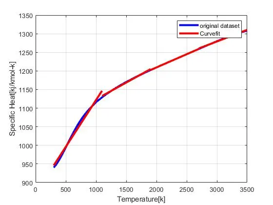
# temperature1 = cp_data(1:800,1); cp_1 = cp_data(1:800,2); the command is used because of the warning occured while increasing the order of polynomial so the order for given temperature date is divided into four where(3200 values is given is divided into four which is called the splitwise polynomial method where temperature1 and cp_1 coordinates are taken ploted by x & y axis.
# temperature2 = cp_data(801:1600,1); cp_2 = cp_data(801:1600,2); the command is used because of the warning occured while increasing the order of polynomial so the order for given temperature date is divided into four where(3200 values is given is divided into four which is called the splitwise polynomial method where temperature2 and cp_2 coordinates are taken ploted by x & y axis.
# temperature3 = cp_data(1601:2400,1); cp_3 = cp_data(1601:2400,2); the command is used because of the warning occured while increasing the order of polynomial so the order for given temperature date is divided into four where(3200 values is given is divided into four which is called the splitwise polynomial method where temperature3 and cp_3 coordinates are taken ploted by x & y axis.
# temperature4 = cp_data(2401:3200,1); cp_4 = cp_data(2401:3200,2); the command is used because of the warning occured while increasing the order of polynomial so the order for given temperature date is divided into four where(3200 values is given is divided into four which is called the splitwise polynomial method where temperature4 and cp_4 coordinates are taken ploted by x & y axis.
# plot(temperature, cp,'linewidth',3,'color','b') the command is used to plot the original data set. where the cp is called on y-axis to represent original value.
# hold on is used adding the new set of values.
# plot(temperature1,predicted_cp_1,'linewidth',3,'color','r') the command is used to plot the curve data set for temperature1 on x-axis and predicted_cp_1 is called on y-axis to represent the first curve set line
# plot(temperature2,predicted_cp_2,'linewidth',3,'color','r') the command is used to plot the curve data set for temperature2 on x-axis and predicted_cp_2 is called on y-axis to represent the first curve set line
# plot(temperature3,predicted_cp_3,'linewidth',3,'color','r') the command is used to plot the curve data set for temperature3 on x-axis and predicted_cp_3 is called on y-axis to represent the first curve set line
# plot(temperature4,predicted_cp_4,'linewidth',3,'color','r') the command is used to plot the curve data set for temperature4 on x-axis and predicted_cp_4 is called on y-axis to represent the first curve set line
# linewidth command represents the width of the line.
# The commands are used to compare the datas between original data and curvefit using splitwise method to plot a graph.
# x-label command is used to represent x-axis.
# y-label command is used to represent y-axis.
# legend command is used for showing the scale in graph.
Plot diagram for splitwise method:
# To measure the Errors:
# m = mean(cp) where cp is already called so m is defined as new variable for the mean
# predicted_cp = [predicted_cp_1, predicted_cp_2, predicted_cp_3, predicted_cp_4]; where all the predicted_cp are set into a array for predicted_cp
# SSR1 =((predicted_cp - (m)).^2); where SSR formula given in article i.e the formula states the sum of predicted cp - means the whole power 2 is given
#SSE1 =((cp_1 - predicted_cp).^2); where SSE is called sum of error where the formula states that cp - predicted_cp the whole power 2 is given to calculate in the article
# SST1 = SSR1 + SSE1; the sum of SSR AND SSE gives the SST
# R_square = SSR1./SST1 to find R^2 the formula is used
# RSME = (SSE1/3200).^0.5 where the SSE/3200 where 3200 is called the given data.
RESULT:
Questions to answer:
1. How to make a curve fit perfectly?
Curve fit helps us to describe our data changes mathematically. once you have the curve fit you can additionally change the data. to make the cut to fit perfectly increase the oder of polynomial for the given data. That helps us to fit the curve perfectly.
2. How to get best fit?
To get the best fit divide the given datas into n numbers and apply the polynomials for all the n numbers to get the best fit.
3. What could be done to improve the cubicfit?
Use different polynomial orders and splitwise polynomial orders for one set of data and other two set of datas for improving the cubicfit.
CONCLUSION:
The code for linear, cubic, and splitwise polynomial for the given data is executed and plotted perfectly.