matlab program for stalagmite mathematical model

AIM:

To solve a program for stalagmite mathematical model for genetic algorithm by using matlab

Objective of the project:

The main objective of the project is to find the minimum value of the stalagmite function with respective to the number of iterations given as input. The work flow of the project starts with creating a 2dimensional mesh where one dimension arrays are created with help of 1D arrays the 2D is created following the flow the stalagmite function is evaluated. for x & y weere we are basically creating an array called input_vector. The stalagmite takes the input vector and calculates the f. By using the given formulas in the question the coding for stalagmite function is to be done to get the minimum value of stalagmite function with different case study to make a 3D graph for gentic algorithm.

Body of content:

study1_code

clear all
close all
clc

%defined our search space
x = linspace(0,0.6,150);
y = linspace(0,0.6,150);
num_cases = 50;

%creating a 2dimensional mesh
[xx,yy] = meshgrid(x,y);

%Evaluating the stalagmite function
for i = 1:length(xx)
    for j = 1:length(yy)
        input_vector(1) = xx(i,j);
        input_vector(2) = yy(i,j);
        f(i,j) = stalagmite(input_vector);
    end
end

tic
%study 1 - statistical behaviour
for i = 1:num_cases
    [inputs, fopt(i)] = ga(@stalagmite, 2);
    xopt(i) = inputs(1);
    yopt(i) = inputs(2);
end
study_time1 = toc
figure(1)
subplot(2,1,1)
hold on
surfc(x,y,-f)
shading interp
plot3(xopt,yopt,-fopt,'marker','o','markersize',5,'markerfacecolor','r')
title('unbounded inputs')
subplot(2,1,2)
plot(fopt)
xlabel('iterations')
ylabel('function maximum')

function code for ga

function A = stalagmite(input_vector)
x = input_vector(1);
y = input_vector(2);
f1 = (sin(5.1*pi*x +0.5)).^6;
f2 = exp(-4*log(2)*((y-0.0667)^2)/0.64);
f3 = (sin(5.1*pi*x +0.5)).^6;
f4 = exp(-4*log(2)*((y-0.0667)^2)/0.64);
A = -(f1*f2*f3*f4);
end

# x = linspace(0,0.6,150); - linspace command is used for providing intervals with a given value, where the value for x and y is given and these are the input arrays of x and y.

# y = linspace(0,0.6,150) - linspace command is used for providing intervals with a given value, where the value for x and y is given and these are the input arrays of x and y.

# num_cases = 50; - num cases is 50 called the genetic algorithm to run for 50 times

# [xx,yy] = meshgrid(x,y); - the command is used to mesh the 2D or 3D plot, where x and y are the axis the plots to meshed.

# for i = 1:length(xx) - for loop is created for repeating the set of values with respective to x-axis.

# for j = 1:length(yy) - for loop is created for repeating the set of values with respective to x-axis.

# input_vector(1) = xx(i,j); - for each value of x basically an array is created called input_vector.

# input_vector(2) = yy(i,j); - for each value of y basically an array is created called input_vector.

# f(i,j) = stalagmite(input_vector); - Where stalagmite is a function. The stalagmite takes the input_vector and calculates the f.

# end - The command must be used when for loop is called.

# tic - the command is used to calculate the operation time performed.

# [inputs, fopt(i)] = ga(@stalagmite, 2); where the study for statistical behaviour is started with inputs and fopt(i) are the variables for the given input. stalagmite is a function a code is written seperately and called for the operation. 2 is the no of variables as inputs.

# xopt(i) = inputs(1); - the x value for the input is wriiten with the variable called xopt.

# yopt(i) = inputs(2); - the y value for the input is wriiten with the variable called yopt.

# end - forloop is called so end must be used

# study_time1 = toc -the command is used to calculate the operation time performed for study1.

# subplot(2,1,1) - The subplot command is used for creating multiple plot with a plot. The 2,1 is the x and y axis with respective to first column.

# hold on - the command is used for adding new elements for showing the graph.

# surfc(x,y,-f) - surfc command is used for creating the surface for the function.

# shading interp - the command is used to plot the 3D graph where the grid on the 3D will be as smooth shading.

# plot3(xopt,yopt,-fopt,'marker','o','markersize',5,'markerfacecolor','r') the command is used for plotting the x,y,z axis in the graph. The marker and markersize command are used to created the size and shape of the maxima.

# title('unbounded inputs') - the command used to represent the graph name.

# subplot(2,1,2) - The subplot command is used for creating multiple plot with a plot. The 2,1 is the x and y axis with respective to second column.

#plot(-fopt) - (-fopt) is given to plot the graph in maxima.

# xlabel('iterations') - xlabel is the command used for creating x-axis name.

# ylabel('function maximum') - ylabel is the command used for creating y-axis name.

Graph for study1:

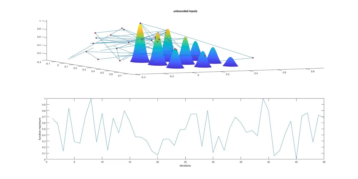
study_time1 = 4.25 secs is the time taken to execute study1.

Result:

The value for x = 0.0668

The value for y = 0.0654

The value for z = 0.998 this is the minimum obtained from x and y.

study2_code

tic
%study 2 -  statistical behaviours with upper and lower bounds
for i = 1:num_cases
    [inputs, fopt(i)] = ga(@stalagmite,2,[],[],[],[],[0;0],[0.6;0.6]);
    xopt(i) = inputs(1);
    yopt(i) = inputs(2);
end
study_time2 = toc
figure(2)
subplot(2,1,1)
surf(x,y,-f)
shading interp
hold on
plot3(xopt, yopt, -fopt,'marker','o','markersize',5,'markerfacecolor','r')
title('bounded inputs')
subplot(2,1,2)
plot(-fopt)
xlabel('iterations')
ylabel('function maximum')

# tic - the command is used to calculate the operation time performed.

# [inputs, fopt(i)] = ga(@stalagmite,2,[],[],[],[],[0;0],[0.6;0.6]); where the study for statistical behaviour is started with inputs and fopt(i) are the variables for the given input. stalagmite is a function a code is written seperately and called for the operation. 2 is the no of variables as inputs, [],[],[],[] are the variable arguments. [0;0],[0.6;0.6] are the xx and yy.

# xopt(i) = inputs(1); - the x value for the input is wriiten with the variable called xopt.

# yopt(i) = inputs(2); - the y value for the input is wriiten with the variable called yopt.

# end - forloop is called so end must be used

# study_time2 = toc -the command is used to calculate the operation time performed for study2.

# subplot(2,1,1) - The subplot command is used for creating multiple plot with a plot. The 2,1 is the x and y axis with respective to first column.

# hold on - the command is used for adding new elements for showing the graph.

# surfc(x,y,-f) - surfc command is used for creating the surface for the function.

# shading interp - the command is used to plot the 3D graph where the grid on the 3D will be as smooth shading.

# plot3(xopt,yopt,-fopt,'marker','o','markersize',5,'markerfacecolor','r') the command is used for plotting the x,y,z axis in the graph. The marker and markersize command are used to created the size and shape of the maxima.

# title('bounded inputs') - the command used to represent the graph name.

# subplot(2,1,2) - The subplot command is used for creating multiple plot with a plot. The 2,1 is the x and y axis with respective to second column.

#plot(-fopt) - (-fopt) is given to plot the graph in maxima.

# xlabel('iterations') - xlabel is the command used for creating x-axis name.

# ylabel('function maximum') - ylabel is the command used for creating y-axis name.

Graph for study_2:

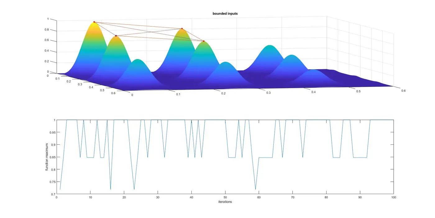
study_time2 = 5.55 secs is the time taken to execute study2.

Result:

The value for x = 0.0668

The value for y = 0.0682

The value for z = 1 this is the minimum obtained from x and y.

study3_code:

%study 3 increasing ga iterations
options = optimoptions('ga')
options = optimoptions(options,'populationsize',500);
tic
for i = 1:num_cases
    [inputs, fopt(i)] = ga(@stalagmite,2,[],[],[],[],[0;0],[0.1;0.1],[],[],options)
    xopt(i) = inputs(1);
    yopt(i) = inputs(2);
end
study_time3 = toc
figure(3)
subplot(2,1,1)
hold on 
surf(x,y,-f)
shading interp
plot3(xopt,yopt,-fopt,'marker','o','markersize',5,'markerfacecolor','r')
title('bounded inputs with increasing ga')
subplot(2,1,2)
plot(-fopt)
xlabel('iterations')
ylabel('function maximum')

# options = optimoptions('ga') - the command is a solver name were used to solve ga

# options = optimoptions(options,'populationsize',500); the command is a solver name where x,y and the value for the population size is given.

# tic - the command is used to calculate the operation time performed.

# [inputs, fopt(i)] = ga(@stalagmite,2,[],[],[],[],[0;0],[0.1;0.1],[],[],options); where the study for statistical behaviour is started with inputs and fopt(i) are the variables for the given input. stalagmite is a function a code is written seperately and called for the operation. 2 is the no of variables as inputs, [],[],[],[] are the variable arguments. [0;0],[0.6;0.6] are the xx and yy and value argument with options solver is used for running the function.

# xopt(i) = inputs(1); - the x value for the input is wriiten with the variable called xopt.

# yopt(i) = inputs(2); - the y value for the input is wriiten with the variable called yopt.

# end - forloop is called so end must be used

# study_time3 = toc -the command is used to calculate the operation time performed for study3.

# subplot(2,1,1) - The subplot command is used for creating multiple plot with a plot. The 2,1 is the x and y axis with respective to first column.

# hold on - the command is used for adding new elements for showing the graph.

# surfc(x,y,-f) - surfc command is used for creating the surface for the function.

# shading interp - the command is used to plot the 3D graph where the grid on the 3D will be as smooth shading.

# plot3(xopt,yopt,-fopt,'marker','o','markersize',5,'markerfacecolor','r') the command is used for plotting the x,y,z axis in the graph. The marker and markersize command are used to created the size and shape of the maxima.

# title('bounded inputs with increasing ga') - the command used to represent the graph name.

# subplot(2,1,2) - The subplot command is used for creating multiple plot with a plot. The 2,1 is the x and y axis with respective to second column.

#plot(-fopt) - (-fopt) is given to plot the graph in maxima.

# xlabel('iterations') - xlabel is the command used for creating x-axis name.

# ylabel('function maximum') - ylabel is the command used for creating y-axis name.

Graph for study_3:

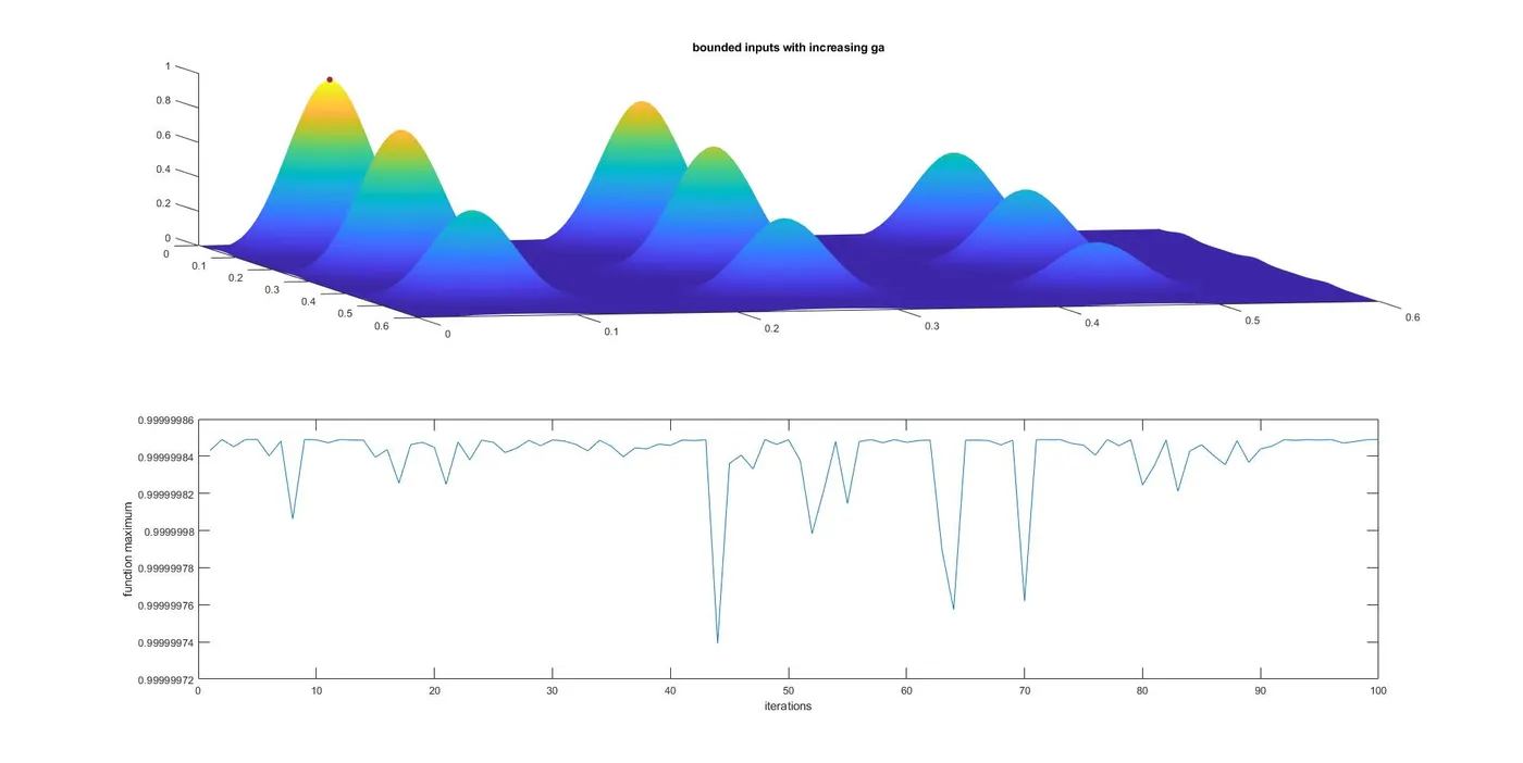
study_time3 = 36.43 secs is the time taken to execute study3.

Result:

The value for x = 0.0684

The value for y = 0.0644

The value for z = 0.9935 this is the minimum obtained from x and y.

Theory about genetic algorithm

# The algorithm works with creating initial population. It creates a sequence of new populations. At each step the algorithm uses the individuals in the current generation to create next generation. It is a optimisation process where search based optimization technique are used in the principles of genetics and natural selection. It is the frequency used to find optimal or non-optimal solutions. The frequency used to solve optimization problems in research, and in machine learning. The process of natural selection starts with the selection of fittest individuals from a population. They produce offspring which inherit the characteristics of the parents and will be added to the next generation. If parents have better fitness, their offspring will be better than parents and have a better chance at surviving. This process keeps on iterating and at the end, a generation with the fittest individuals will be found.

In a genetic algorithm, a population of candidate solutions (called individuals, creatures, or phenotypes) to an optimization problem is evolved toward better solutions. Each candidate solution has a set of properties (its chromosomes or genotype) which can be mutated and altered; traditionally, solutions are represented in binary as strings of 0s and 1s, but other encodings are also possible.

The evolution usually starts from a population of randomly generated individuals, and is an iterative process, with the population in each iteration called a generation. In each generation, the fitness of every individual in the population is evaluated; the fitness is usually the value of the objective function in the optimization problem being solved. The more fit individuals are stochastically selected from the current population, and each individual's genome is modified (recombined and possibly randomly mutated) to form a new generation. The new generation of candidate solutions is then used in the next iteration of the algorithm. Commonly, the algorithm terminates when either a maximum number of generations has been produced, or a satisfactory fitness level has been reached for the population.

A typical genetic algorithm requires:

# A genetic representation of the solution domain,

# A fitness function to evaluate the solution domain.

A standard representation of each candidate solution is as an array of bits. Arrays of other types and structures can be used in essentially the same way. The main property that makes these genetic representations convenient is that their parts are easily aligned due to their fixed size, which facilitates simple crossover operations. Variable length representations may also be used, but crossover implementation is more complex in this case. Tree-like representations are explored in genetic programming and graph-form representations are explored in evolutionary programming; a mix of both linear chromosomes and trees is explored in gene expression programming.

How does the ga work?

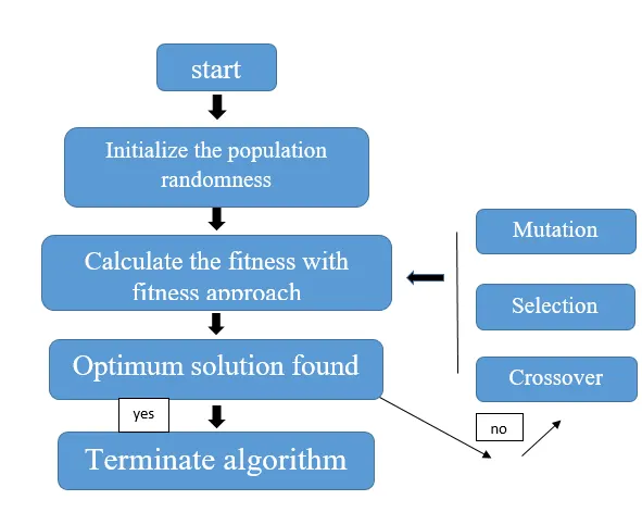
GA optimisation starts with population initialization. Population is the number of sample data points taken to perform the genetic algorithm operation. The sample data points undergo three steps. They are

# Selection.

# Crossover.

# Mutuation.

* SELECTION: (The process is to select the highly fit)

Selection is the stage of a genetic algorithm in which individual genomes are chosen from a population for later breeding (using the crossover operator).

A generic selection procedure may be implemented as follows:

# The fitness function is evaluated for each individual, providing fitness values, which are then normalized. Normalization means dividing the fitness value of each individual by the sum of all fitness values, so that the sum of all resulting fitness values equals 1.

# Accumulated normalized fitness values are computed: the accumulated fitness value of an individual is the sum of its own fitness value plus the fitness values of all the previous individuals; the accumulated fitness of the last individual should be 1, otherwise something went wrong in the normalization step.

# A random number R between 0 and 1 is chosen.

# The selected individual is the first one whose accumulated normalized value is greater than or equal to R.

* CROSSOVER: (Process of taking two parents solutions and producing the child from them)

# The crossover operator is analogous to reproduction and biological crossover. In this more than one parent is selected and one or more off-springs are produced using the genetic material of the parents. Crossover is usually applied in a GA with a high probability.

# n this section we will discuss some of the most popularly used crossover operators. It is to be noted that these crossover operators are very generic and the GA Designer might choose to implement a problem-specific crossover operator as well.

One Point Crossover
# In this one-point crossover, a random crossover point is selected and the tails of its two parents are swapped to get new off-springs.

Multi Point Crossover
# Multi point crossover is a generalization of the one-point crossover wherein alternating segments are swapped to get new off-springs.

* MUTUATION

# Mutation is a genetic operator used to maintain genetic diversity from one generation of a population of genetic algorithm chromosomes to the next. Mutation alters one or more gene values in a chromosome from its initial state. In mutation, the solution may change entirely from the previous solution. Hence GA can come to a better solution by using mutation.

# Mutation occurs during evolution according to a user-definable mutation probability. This probability should be set low. If it is set too high, the search will turn into a primitive random search.

# The classic example of a mutation operator involves a probability that an arbitrary bit in a genetic sequence will be flipped from its original state. A common method of implementing the mutation operator involves generating a random variable for each bit in a sequence. This random variable tells whether or not a particular bit will be flipped. Other types are inversion and floating point mutation. When the gene encoding is restrictive as in permutation problems, mutations are swaps, inversions, and scrambles.

# The purpose of mutation in GAs is to introduce diversity into the sampled population. Mutation operators are used in an attempt to avoid local minima by preventing the population of chromosomes from becoming too similar to each other, thus slowing or even stopping convergence to the global optimum.

# This reasoning also leads most GA systems to avoid only taking the fittest of the population in generating the next generation, but rather selecting a random (or semi-random) set with a weighting toward those that are fitter.

* FITNESS FUNCTION:

# Takes the solution as input and produces the suitability of the solution as the output. This evaluates how to close the solution is to the solution to the optimal solution os desired problem

GA used areas:

# Optimization - where to maximize (or) minimize a given objective function value under a given set of constraints.

# Economics - Characterize various economic models like cobweb model, game theory equlibrium resolution, asset, pricing.

# Netral network - recurrent netral networks

# Image processing - (DIP) takes as well like dense pixel matching.

syntax for ga