Project - Data Handling and Interpolation
AIM :
To perform the Interpolation from the given current and voltage values to be read by Excel spreadsheet and to generate the interactive plot for the interpolated data and also to compute these above current and voltage values to store them into a text file.
Interpolation
Interpolation is a method of deriving a simple function from the given discrete data set such that the function passes through the provided data points. This helps to determine the data points in between the given data ones. This method is always needed to compute the value of a function for an intermediate value of the independent function. In short, interpolation is a process of determining the unknown values that lie in between the known data points. It is mostly used to predict the unknown values for any geographical-related data points such as noise level, rainfall, elevation, and so on.
Types of interpolation methods are :
1. Linear interpolation
2. Nearest neighbor interpolation or Piecewise constant interpolation
3. Polynomial interpolation
4. Spline interpolation
5. Mimetic interpolation
The Most popular and widely used methods are Linear and spline interpolation
1. Linear interpolation
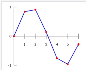
The Linear Interpolation Method applies a distinct linear polynomial between each pair of the given data points for the curves, or within the sets of three points
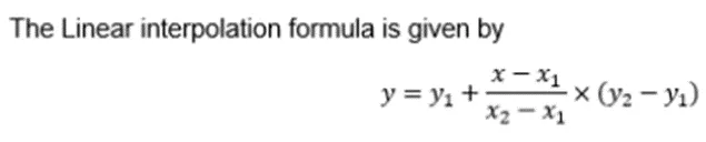
The unknown value on the data points can be found using the linear interpolation formula
2. Polynomial interpolation
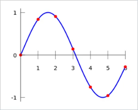
Polynomial interpolation is a generalization of linear interpolation. Note that the linear interpolant is a linear function. We now replace this interpolant with a polynomial of a higher degree.
if we have n data points, there is exactly one polynomial of degree at most n−1 going through all the data points. The interpolation error is proportional to the distance between the data points to the power n. Furthermore, the interpolant is a polynomial and thus infinitely differentiable. So, we see that polynomial interpolation overcomes most of the problems of linear interpolation.
3. Spline Interpolation
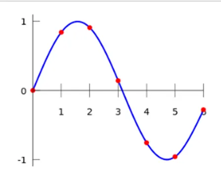
The linear interpolation uses a linear function for each of the intervals [xk,xk+1]. Spline interpolation uses low-degree polynomials in each of the intervals, and chooses the polynomial pieces such that they fit smoothly together. The resulting function is called a spline.
Interp1
It is used in 1-D data interpolation.
Syntax
vq = interp1(x,v,xq,method,extrapolation)
vq = interp1(v,xq,method,extrapolation)
vq = interp1(x,v,xq) returns interpolated values of a 1-D function at specific query points using linear interpolation. Vector x contains the sample points, and v contains the corresponding values, v(x). Vector xq contains the coordinates of the query points.
If you have multiple sets of data that are sampled at the same point coordinates, then you can pass v as an array. Each column of array v contains a different set of 1-D sample values.
vq = interp1(x,v,xq,method) specifies an alternative interpolation method: 'linear', 'nearest', 'next', 'previous', 'pchip', 'cubic', 'v5cubic', 'makima', or 'spline'. The default method is 'linear'.
vq = interp1(x,v,xq,method,extrapolation) specifies a strategy for evaluating points that lie outside the domain of x. Set extrapolation to 'extrap' when you want to use the method algorithm for extrapolation. Alternatively, you can specify a scalar value, in which case, interp1 returns that value for all points outside the domain of x.
vq = interp1(v,xq) returns interpolated values and assumes a default set of sample point coordinates. The default points are the sequence of numbers from 1 to n, where n depends on the shape of v:
- When v is a vector, the default points are 1:length(v).
- When v is an array, the default points are 1:size(v,1).
vq = interp1(v,xq,method) specifies any of the alternative interpolation methods and uses the default sample points.
vq = interp1(v,xq,method,extrapolation) specifies an extrapolation strategy and uses the default sample points.
pp = interp1(x,v,method,'pp') returns the piecewise polynomial form of v(x) using the method algorithm.
Interp2
It is used in interpolation for 2-D gridded data in meshgrid format.
Syntax
Vq = interp2(___,method,extrapval)
Vq = interp2(X,Y,V,Xq,Yq) returns interpolated values of a function of two variables at specific query points using linear interpolation. The results always pass through the original sampling of the function. X and Y contain the coordinates of the sample points. V contains the corresponding function values at each sample point. Xq and Yq contain the coordinates of the query points.
Vq = interp2(V,Xq,Yq) assumes a default grid of sample points. The default grid points cover the rectangular region, X=1:n and Y=1:m, where [m,n] = size(V). Use this syntax when you want to conserve memory and are not concerned about the absolute distances between points.
Vq = interp2(V) returns the interpolated values on a refined grid formed by dividing the interval between sample values once in each dimension.
Vq = interp2(V,k) returns the interpolated values on a refined grid formed by repeatedly halving the intervals k times in each dimension. This results in 2^k-1 interpolated points between sample values.
Vq = interp2(___,method) specifies an alternative interpolation method: 'linear', 'nearest', 'cubic', 'makima', or 'spline'. The default method is 'linear'.
Vq = interp2(___,method,extrapval) also specifies extrapval, a scalar value that is assigned to all queries that lie outside the domain of the sample points.
If you omit the extrapval argument for queries outside the domain of the sample points, then based on the method argument interp2 returns one of the following:
- Extrapolated values for the 'spline'and 'makima' methods
- NaNvalues for other interpolation methods
#PROGRAM CODE
%% performing the interpolation
clear all
close all
clc
VI = xlsread('VI.xlsx');
V = VI(:,1);
I = VI(:,2);
VI = [-17.3:0.1:0.9]; % The range in which interpolation carried out
V1 = interp1(V,I,VI); % Performing linear interpolation
V2 = interp1(V,I,VI,'spline'); % Performing Spline interpolation
figure(1)
plot(V,I,'o',VI,V1,':.','Linewidth',2); grid; % plot for linear interpolation
xlabel("Voltage(V)"); % labelling voltage in x-axis
ylabel("Current(I)"); % labelling current in the Y-axis
title("Linear interpolation"); % To give the title on the plot
legend('Actual value','interpolated value','Location','Southeast');
figure(2)
plot(V,I,'b',VI,V2,':.','Linewidth',2); grid; % Performing Spline interpolation plot
xlabel("Voltage(V)");
ylabel("Current(I)");
title("Spline interpolation");
legend('Actual value','interpolated value','Location','Northwest');
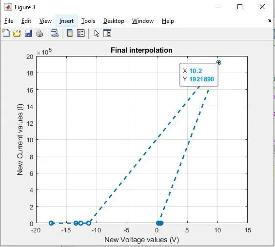
%% Final interpolation
VV1 = [-17.5 -13.4 -12.6 -11.3 10.2 0.25 0.5 0.61 0.66]; % taking new voltage values
VV2 = interp1(V,I,VV1,'spline'); % Performing Spline interpolation
figure(3)
plot(VV1,VV2,'o--','Linewidth',2); grid; % Plotting Linear Interpolation
xlabel('New Voltage values (V)');
ylabel('New Current values (I)');
title("Final interpolation");
%% Saving Output Files
VI_output = [VV1;VV2];
fileID = fopen('VI_linear.txt','w'); % Writing to text file
fprintf(fileID,'%6s %12s\n','Voltage','Current'); % Writing title of the columns
fprintf(fileID,'%6.2f %12.2f\n',V1); % Writing Output values
fclose(fileID);fileID = fopen('VI_spline.txt','w'); % Writing to text file
fprintf(fileID,'%6s %12s\n','Voltage','Current'); % Writing title of the columns
fprintf(fileID,'%6.2f %12.2f\n',V2); % Writing Output values
fclose(fileID);
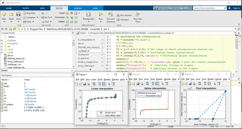
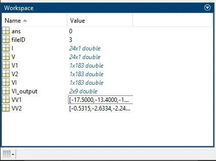
WORKSPACE RESULTS
INTERPOLATED DATA PLOTS
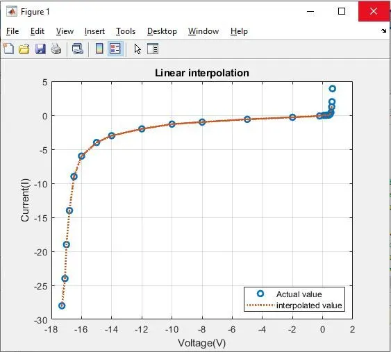
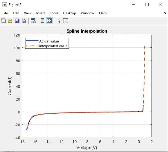
RESULTS
- Excel file was read in Matlab and performed linear and spline interpolation.
- After a comparison of the two interpolation methods, it was found that the spline interpolation is more accurate.
- Generated the plot of the interpolated data and saved the data in a text file.
REFERENCES