Project 2 - Rankine cycle Simulator

RANKINE CYCLE SIMULATOR

Aim:

Creation of Rankine cycle simulator from given input and reading the data from a standard thermodynamic library of steam table.

Objective :

1. To Simulate a Rankine cycle using Matlab.
2. Extracting Steam and water properties from XSteam data (IAPWS IF - 97 standard)
3. Calculate all the state points of the cycle based on User inputs.
4. Plotting the T vs s and H vs s plots for the given input.

Rankine Cycle :

• Rankine cycle is an idealized thermodynamic cycle or heat engine in which a fuel is used to produce heat within a boiler , converting water into steam which then expands through a turbine producing useful wok . This process was developed in 1859 by scottish engineer william J.m Rankine . It is a cycle which converts heat into mechanical energy which usually is converted into electrical energy.

1. In this project an idealized cycle is simulated. Hence neglecting losses.
2. The Rankine cycle is derived from the Carnot cycle. its power depends on the temperature difference between the heat source and a cold source. The more the difference the more mechanical power can be efficiently extracted out of heat energy.
3. Since ideal cycles are only in theory, the Efficiency of Rankine cycle is limited by high heat of vaporization of the working fluid , friction losses etc.
4. Water is usually the fluid of choice due to its favorable properties, such as its non-toxic and unreactive chemistry, abundance, and low cost, as well as its thermodynamic properties. By condensing the working steam vapor to a liquid the pressure at the turbine outlet is lowered and the energy required by the feed pump consumes only 1% to 3% of the turbine output power and these factors contribute to a higher efficiency for the cycle. The benefit of this is offset by the low temperatures of steam admitted to the turbine

Processes and Working :

There are four processes in the Rankine cycle (order may be varied):

1. Process 1-2 : Isentropic Expansion in the turbine.
2. Process 2-3 : Constant pressure Heat rejection in the condenser
3. Process 3-4 : Isentropic compression in the pump
4. Process 4-1 : Constant pressure heat addition in the boiler

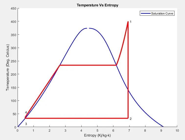
( This Plot is obtained from the Matlab program, T vs S plot )

• Working of the Rankine cycle simulator

1. In process 1-2 , The dry saturated vapour expands through a turbine, generating power. This decreases the temperature and pressure of the vapour, and some condensation may occur.
2. Process 2-3 , The vapor-liquid mixture leaving the turbine (2) is condensed at low pressure, usually in a surface condenser using cooling water. In well designed and maintained condensers, the pressure of the vapor is well below atmospheric pressure, approaching the saturation pressure of the operating fluid at the cooling water temperature.
3. Process 3-4 , The pressure of the condensate is raised in the feed pump. Because of the low specific volume of liquids, the pump work is relatively small and often neglected in thermodynamic calculations.
4. Process 4-1 , High pressure liquid enters the boiler from the feed pump (4) and is heated to the saturation temperature (on the saturation curve). Further addition of energy causes evaporation of the liquid until it is fully converted to saturated steam (1) or superheated (1).

Matlab Project Program:

The code for Rankine Cycle Simulator is given as:

clear all
close all
clc

% Rankine Cycle Simulator

fprintf(' Rankine Cycle\n ')
fprintf('1-2 is Isentropic Expansion in Turbine\n')
fprintf(' 2-3 is constant pressure heat removal\n')
fprintf(' 3-4 is Isentropic Compression in Pump \n')
fprintf(' 4-1 Constant pressure Heat addition in Boiler\n')

% Entering the input data for calculation of state points
p1 = 50;        %Pressure at Turbine Inlet
T1 = 500;       %Temperature at Turbine Inlet
p2 = 5;      %Pressure at Condenser

% Taking data from Xsteam file for State point 1
h1 = XSteam('h_pT', p1, T1);        % Enthaply at pressure and Temp 1
s1 = XSteam('s_pT', p1, T1);        % Entropy at pressure and Temp 1

% Taking data from Xsteam file for State point 2
s2 = s1;                            % Because of Isentropic Expansion
sf2 = XSteam('sL_p', p2);           % Saturated liquid entropy at pressure 2
sg2 = XSteam('sV_p', p2);           % Saturated vapour entropy at pressure 2
x2 = (s2-sf2)/(sg2-sf2);            % Vapour Fraction at state point 2
hf2 = XSteam('hL_p', p2);           % Saturated liquid Enthalpy at pressure 2
hg2 = XSteam('hV_p', p2);           % Saturated vapour Enthalpy at pressure 2
h2 = hf2 + (x2*(hg2-hf2));          % Enthalpy at state point 2

% Taking data from Xsteam file for state point 3
p3 = p2;                            % Constant Pressure heat removal process
s3 = XSteam('sL_p', p3);            % Saturated liquid entropy at Pressure 3
h3 = XSteam('hL_p', p3);            % Saturated liquid Enthalpy at Pressure 3

% Taking data from Xsteam file for State point 4
s4 = s3;                            % Isentropic Compression process
p4 = p1;                            % Constant Pressure heat rejection

% Work done in Turbine for the rankine cycle
W_T = h1-h2;

% Work done required for pump
v3 = XSteam('vL_p',p3);             % Saturated Liquid Vapour at pressure 3
W_P = v3*(p4-p3)*100;               % Work done for pump
h4 = h3 - W_P;                      % Enthalpy at State point 4

% Net work done for Rankine Cycle
W_net = W_T - W_P;

% Heat Addition to System
Q_in = h1-h4;

% Heat Rejection from System
Q_out = h2-h3;

% Thermal Efficiency of Rankine Cycle
T_eff = (W_net/Q_in)*100;

%specific steam consumption  = (Mass flow rate / Net work done)
Sp_S = (3600/W_net);

% Calculation of Temperature at All state Point 2, 3 and 4
T3 = XSteam('Tsat_p',p3);           % Saturation Temperature at Pressure 3
T2 = T3;                            % Becuase of Constant Pressure Heat addition
Cp4 = XSteam('Cp_ps',p4,s4);        % Specific isobaric heat capacity
Cv4 = XSteam('Cv_ps',p4,s4);        % Specific isochoric heat capacity
k = Cp4/Cv4;
T4 = T3/((p3/p4)^((k-1)/k));        % Temperature at State point 4

% Calculation of Other constant for saturated liquid and Vapour
T6 = XSteam('Tsat_p', p1);          % Saturated Temperature at Pressure 1
s5 = XSteam('sL_p', p1);            % Saturated Liquid entropy at pressure 1
s6 = XSteam('sV_p', p1);            % Saturated Vapour entropy at Pressure 1
h5 = XSteam('hL_p', p1);            % Saturated Liquid Enthalpy at Pressure 1
h6 = XSteam('hV_p', p1);            % Saturated Vapour Enthalpy at pressure 1
T5 = T6;

%Plotting for Saturation Line
T = linspace(1,560,1000);
for i = 1:length(T)
    sf(i) = XSteam('sL_T' ,T(i));   % Saturated Liquid Entropy
    sg(i) = XSteam('sV_T' ,T(i));   % Saturated Vapour Entropy
    hf(i) = XSteam('hL_T' ,T(i));   % Saturated Liquid Enthalpy
    hg(i) = XSteam('hV_T' ,T(i));   % Saturated Vapour Enthalpy
    
end

% Plotting T-S Diagram for Rankine Cycle
figure(1)
hold on
plot(sf,T,'color','r','linewidth',2)
plot(sg,T,'color','r','linewidth',2)
plot([s1 s2],[T1 T2], 'color', 'g', 'linewidth',2.5)
plot([s2 s3],[T2 T3], 'color', 'g', 'linewidth',2.5)
plot([s3 s4],[T3 T4], 'color', 'g', 'linewidth',2.5)
plot([s4 s5],[T4 T5], 'color', 'g', 'linewidth',2.5)
plot([s5 s6],[T5 T6], 'color', 'g', 'linewidth',2.5)
s_1 = linspace(s6,s1,1000);
for j = 1:length(s_1)
    Tc(j) = XSteam('T_ps',p1,s_1(j));
end
plot(s_1,Tc,'color','g','linewidth',2.5)
text(s1+0.1, T1, '1')
text(s2+0.1, T2, '2')
text(s3, T3-20, '3')
text(s4, T4+20, '4')
title('Temperature Vs Entropy')
xlabel('Entropy (Kj/kg-k)')
ylabel('Temeperature (Deg. Celcius)')
legend('Saturation Curve')

% Plotting H-S Diagram for Rankine Cycle
figure(2)
hold on
plot(sf,hf,'color','r','linewidth',2)
plot(sg,hg,'color','r','linewidth',2)
plot([s1 s2],[h1 h2],'color','g','linewidth',2.5)
plot([s2 s3],[h2 h3],'color','g','linewidth',2.5)
plot([s3 s4],[h3 h4],'color','g','linewidth',2.5)
hc = linspace(h4,h5,100);
for k = 1:length(hc)
    s_c(k) = XSteam('s_ph',p1,hc(k));
end
plot(s_c,hc,'color','g','linewidth',2.5)
plot([s5 s6],[h5 h6],'color','g','linewidth',2.5)
for l = 1:length(s_1)
    h_c(l) = XSteam('h_ps',p1,s_1(l));
end
plot(s_1,h_c,'color','g','linewidth',2.5)
text(s1+0.1,h1,'1')
text(s2+0.1,h2,'2')
text(s3,h3-100,'3')
text(s4,h4+200,'4')
title('Enthalpy Vs Entropy')
xlabel('Entropy (Kj/kg-k)')
ylabel('Enthalpy (KJ/Kg)')
legend('Saturation Curve')

% Displaying Results in Command window
disp('Results of Rankine Cycle')
fprintf('At state point 1\t\t\t\t\t')
fprintf('At state Point 2\n')
fprintf('P1 = %10f in Bar\t\t\t\t',p1);
fprintf('P2 = %10f in Bar\n',p2);
fprintf('T1 = %11f in Deg.Celcius\t\t',T1);
fprintf('T2 = %11f in Deg.Celcius\n',T2);
fprintf('H1 = %12f in KJ/Kg\t\t\t',h1);
fprintf('H2 = %12f in KJ/Kg\n',h2);
fprintf('S1 = %9f in KJ/Kg-k\t\t\t',s1);
fprintf('S2 = %9f in KJ/Kg-k\n',s2);
fprintf('\n')
fprintf('At state point 3\t\t\t\t\t')
fprintf('At state Point 4\n')
fprintf('P3 = %10f in Bar\t\t\t\t',p3);
fprintf('P4 = %10f in Bar\n',p4);
fprintf('T3 = %11f in Deg.Celcius\t\t',T3);
fprintf('T4 = %11f in Deg.Celcius\n',T4);
fprintf('H3 = %12f in KJ/Kg\t\t\t',h3);
fprintf('H4 = %12f in KJ/Kg\n',h4);
fprintf('S3 = %9f in KJ/Kg-k\t\t\t',s3);
fprintf('S4 = %9f in KJ/Kg-k\n',s4);
fprintf('\n')
fprintf('Turbine Work Done = %14f in KJ/Kg\n',W_T)
fprintf('Pump Work Done = %15f in KJ/Kg\n',W_P)
fprintf('Net Work Done  = %17f in KJ/Kg\n',W_net)
fprintf('Thermal Efficiency = %13f in percent\n',T_eff)
fprintf('Sp. Steam Consumption = %f in KJ/Kw\n',Sp_S) 

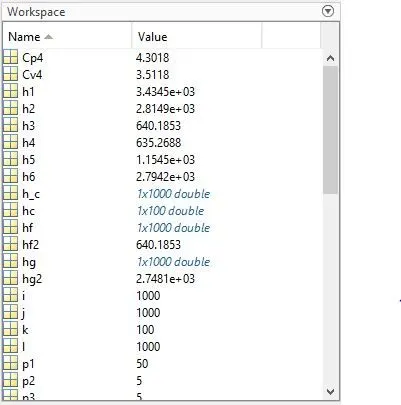
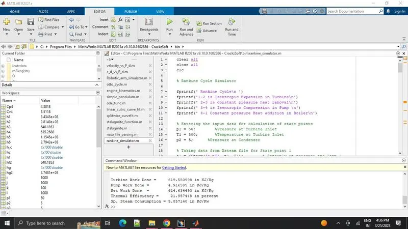
Workspace:

Explanation of Code:

1. The creation of the Rankine cycle simulator starts with some input values that are required to calculate the other state point in cycle eventually.
2. The Rankine cycle process is displayed in the command window and then inputs are entered which are inlet pressure for turbine, temperature at turbine inlet and pressure at condenser.
3. Then we are using XSteam function file for reading state point. First, we get the value of enthalpy and entropy at state point 1 from the XSteam function file.
4. As process from 1-2 is isentropic compression the entropy at point 1 is equal to point 2. The term ‘(s_pT, p1, T1)’ refers to entropy at pressure and temperature point 1.
5. The term ‘sg’ and ‘sf’ are referred to saturated liquid and saturated vapor entropy respectively. This value is used to calculate other function according to mathematical relations.
6. Similarly, other points are taken from XSteam function file which are necessary to calculate other parameters. After that work done in turbine and pump are calculated for further getting the net work done Rankine cycle.
7. After calculating the net work done the efficiency of the Rankine cycle is calculated along with specific steam consumption which is steam consumed by a locomotive cylinder per unit of output of work done.
8. Then temperature at each point of cycle is calculated using input taken from start of the program and data taken from XSteam file. For given temperature range from lower to higher entropy points are calculated to create the T-S plot. Similarly, another for loop is used to create the saturation curve in each plot.
9. Then plotting is done respectively for T-s and H-s graph in Rankine cycle and each state point value has been put in command window.

Inference of Plot:

To make the graph more deliberate we are changing some values in the inputs by increasing the inlet pressure and temperature along with condenser pressure also which results in the following graphs.

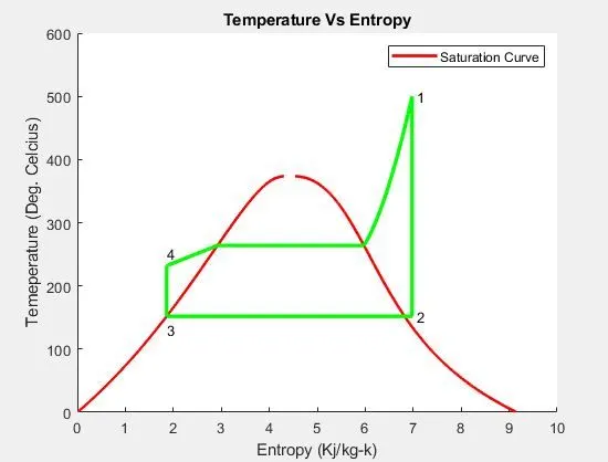
From the above diagram as we can see along the saturation curve point 1 start with turbine from which heat rejection is started which is again an isentropic process. The steam is get cooled in condenser and in form of saturated liquid as it is under the curve. Then it was pumped to enter in boiler where its temperature is increased to change it from saturated liquid to saturated vapor form.

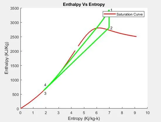
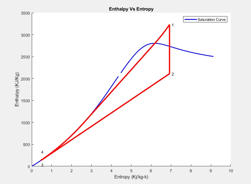
As we can see from above plot the steam entropy changes during the process with respect to enthalpy. As the heat added in the system the entropy has been increased and similarly as the heat removed from the system the entropy drops with similar rates.

For the parameters given in the challenge, the graph will look like this:

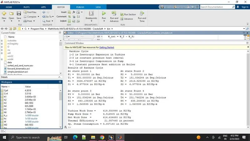
The values for the state point in command windows are given as:

For Inlet pressure in Turbine as = 50 bar

Inlet temperature in Turbine = 500 deg.cel

Pressure in condenser = 5 bar

For Input given in challeng:

For Inlet pressure in Turbine as = 30 bar

Inlet temperature in Turbine = 400 deg.cel

Pressure in condenser = 0.05 bar

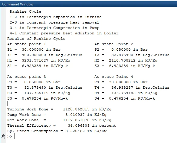
From the two different input values it is seen that increasing the pressure and temperature in the Turbine results in lowering the efficiency of the Rankine cycle.

Errors:

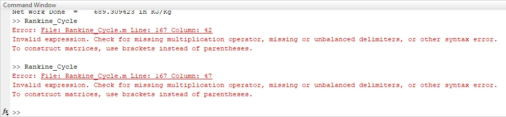
This error is mostly coming because of entering the wrong keywords for saturated entropy and enthalpy from XSteam function file.

Conclusion:

So, we have created the Rankine cycle simulator for the given input, in which we have taken the data from XSteam function file.

References:

1) https://www.nuclear-power.net/nuclear-engineering/thermodynamics/thermodynamic-cycles/rankine-cycle-steam-turbine-cycle/theory-of-rankine-cycle-equations-and-calculation/

2) https://in.mathworks.com/matlabcentral/answers/12855-newlines-and-spaces-in-strings