Week 4.1 - Solving second order ODEs

SIMPLE PENDULUM MOTION WITH DAMPING

AIM:

To write a program to solve the Ordinary differential equation (ODE) for the equation of motion of a simple pendulum with damping and to create a movie animation for the motion of the pendulum.

THEORY:

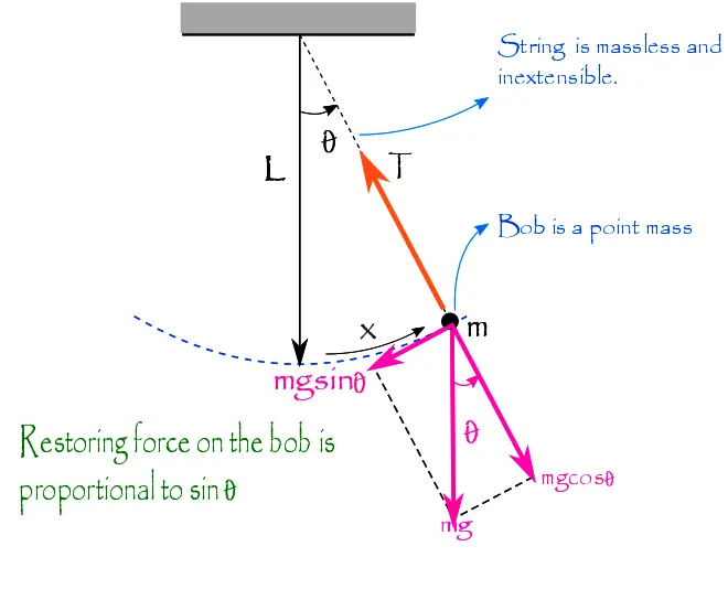
• The simple pendulum is formed of a light, stiff, inextensible rod of length 'l' with a Bob of mass 'm'. its position with respect to time t can be described merely by the angle θ (measured against a reference line, usually taken as the vertical line straight down).
• The fact that its position can be described by using only variables means that a simple pendulum has only one degree of freedom.
• An example of a damped simple harmonic motion is a simple pendulum.

GOVERNING EQUATIONS:

The way the pendulum moves depends on Newton's second law of motion, when this law has been written, we get second-order ordinary differential equations (ode) that describe the position of the "ball" with respect to time.

The second-order ode below represents the equation of motion of a simple pendulum with damping

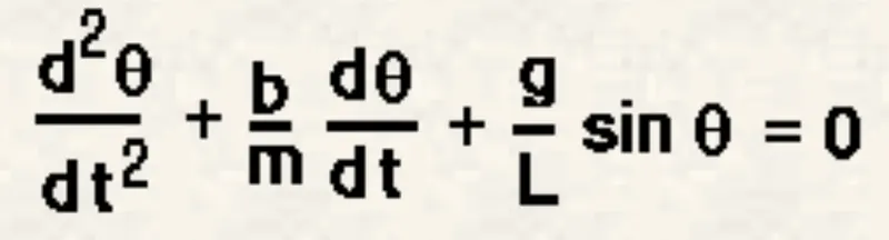
where,

• b = damping coefficient,
• m = mass of the Bob in kg
• g = gravity in m/s^2
• l = length of the pendulum in m.

In order to solve the equation of motion for the pendulum and as the ode is of higher order we break the 2nd-order ode into a series of 1st-order ode.

The final ode equations to solve are represented as :

d^2θ/dt^2 + b/m*dθ/dt + g/L*sinθ = 0

In order to solve ode's, we need to break down second-order ode into single-order ode.

Simplifying the above equation,

OBJECTIVES:

1. To Create a program that solves the ODE for the equation of motion of a simple pendulum with damping and describes the transient behavior of the system.
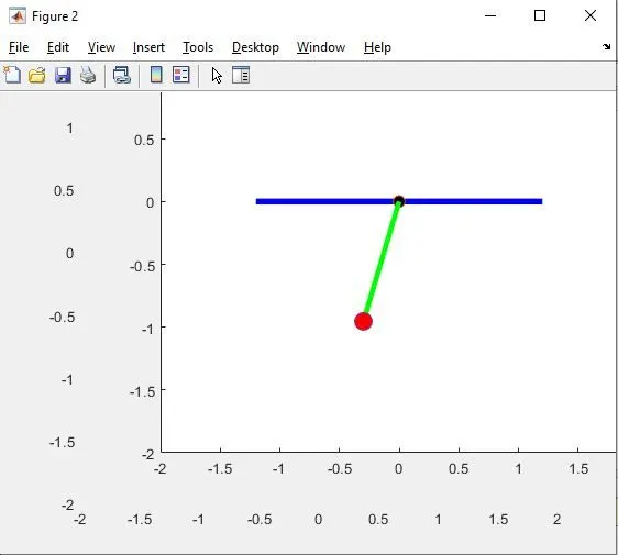
2. To get the position of the pendulum as a function of time and use that data to animate the motion of the pendulum

Main Code:

% A program to simulate the transient behavior of a Simple Pendulum 
clear all
close all
clc

% inputs 
b = 0.05;   % Damping coefficient
g = 9.81;   % gravity in m/s^2
l = 1;      % length of the pendulum in meter
m = 1;      % mass of the Bob in kg

% initial condition
theta_0 = [0;3];      % {initial disp, initial velocity}

% time interval
t_span = linspace(0,20,500);     

% solving ODE
[t,results] = ode45(@(t,theta) ode_func(t,theta,b,g,l,m),t_span, theta_0);

% Plotting
figure(1)
plot(t,results(:,1))
hold on
plot(t,results(:,2))
hold on
xlabel('Time in sec')
ylabel('Plot for Displacement and Velocity')
legend('Displacement','Velocity')

% plot for different positions of pendulum for movie animation
counter_ct = 1;
THETA_disp = results(:,1);

for i = 1:length(THETA_disp)
    THETA_0 = THETA_disp(i);
    
    % Asigning the co-ordinates
    x0 = 0;
    y0 = 0;
    
    x1 = l*sin(THETA_0);
    y1 = -l*cos(THETA_0);
    
    % Plotting the pendulum for motion
    figure(2)
    plot([-1.2 1.2],[0 0], 'linewidth',4, 'color','b')
    hold on 
    plot([0 0],[0 0], 'o', 'markerfacecolor','k', 'markersize',8)
    hold on
    plot([x0 x1],[y0 y1], 'linewidth',3.5, 'color','g')
    hold on 
    plot(x1,y1,'o', 'markersize',12,'markerfacecolor','r')
    hold off
    axis([-2 2 -2 1])
    pause(0.01)
    
    E(counter_ct) = getframe(gcf);
    counter_ct = counter_ct + 1;
end

% Creating a movie and saving it in file
movie(E)
videofie = VideoWriter('simple pendulum.avi', 'Uncompressed AVI')
open(videofile)
writeVideo(videofile,E)
close(videofile)

Code for Function call:

% A program for calling function 

function [dtheta_dt] = ode_func(t,theta,b,g,l,m)
  
  theta1 = theta(1);
  theta2 = theta(2);
  
  dtheta1_dt = theta2;
  
  dtheta2_dt = -b/m*theta2 - (g/l)*sin(theta1);
  
  dtheta_dt = [dtheta1_dt; dtheta2_dt];
  
end

Detail explanation of each step of the program:

1. In the first step Input and initial condition of a simple pendulum are fed.

2. Then the program is written to solve the ODE in which Matlab inbuilt function (ode45) is used with constant theta, t, and another function is used, which is defined separately in the function program.

3. In the next step result of the solved ODE is plotted w.r.t time using the plot command.

4. Now iteration of co-ordinate is fed using for loop to create animation.

5. Then plot command is used to plot the pendulum string and bob.

6. In the next step, the move command is used to create an animated video of the oscillating pendulum.

Output:

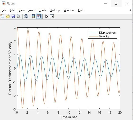
• The output obtained is a graphical representation of velocity and displacement curve w.r.t Time.
• Angular Displacement and Angular Velocity plots were generated for a time range of 20 secs.

Conclusion for the above Output plot:

From the above plot we have understood the frequency of angular Displacement(blue color) along with the angular velocity decreases with increases in the time period (0-20 sec)

Various errors are faced while programming as followed:

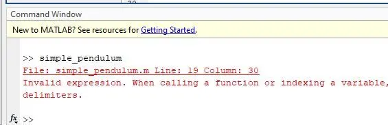
The above error occurred due to incorrect inputs given when calling the function to pass the input arguments hence correcting the inputs given

Correcting the spelling mistakes from the function program by reviewing each line of the program.

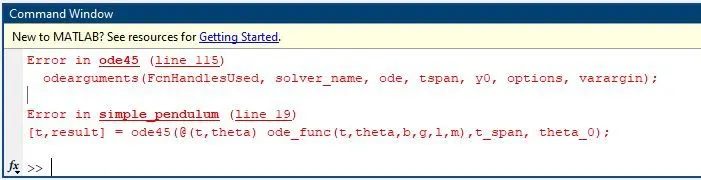
• The error occurred in ode45 inbuilt Matlab ode solver due to giving wrong governing equations
• The governing equation is given below,

dtheta2_dt = -b/m*theta2 - g/L*sin(theta1)

Final Conclusion:

Thus, the simulation of the transient behavior of a simple pendulum is successfully created by using a program in Matlab.

For Animated Video:

https://youtu.be/vo8uqfqMkDw