Project 1 - Parsing NASA thermodynamic data

Aim:

 To write a code in MATLAB to parse the NASA thermodynamic data file and calculate the thermodynamic properties of various gas species.

Objective:

• To develop a function that extracts the 14 coefficients and calculates the enthalpy, entropy, and specific heats for all the species in the data file.
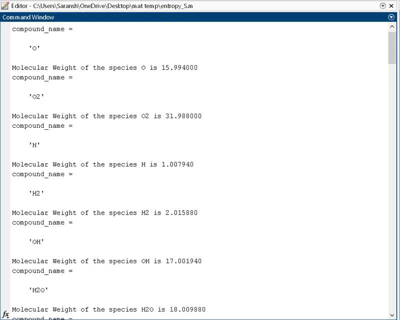
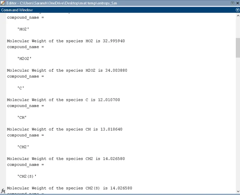
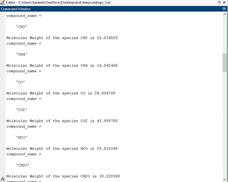
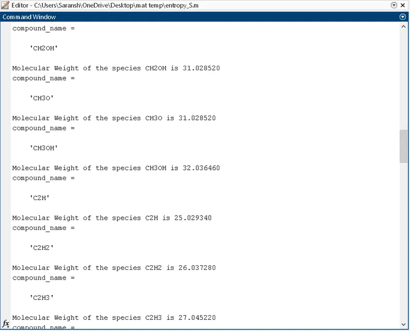
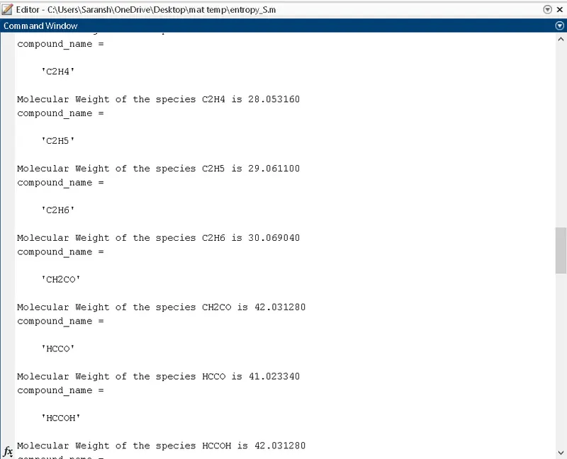
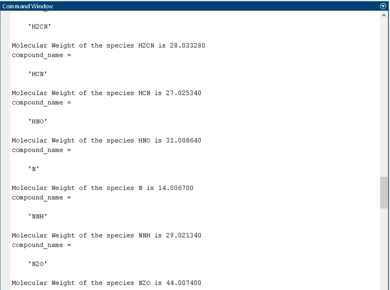
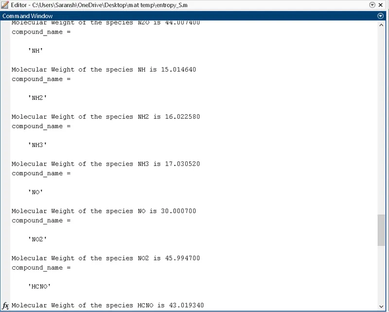
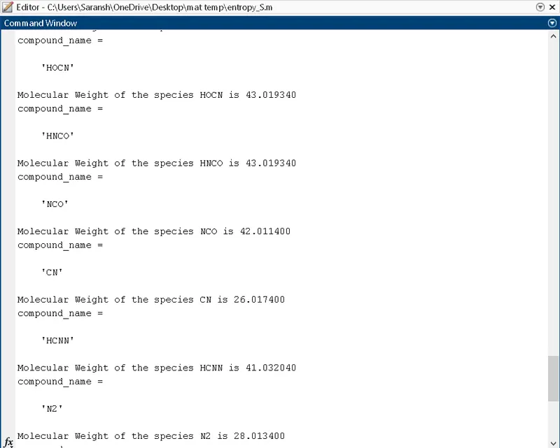
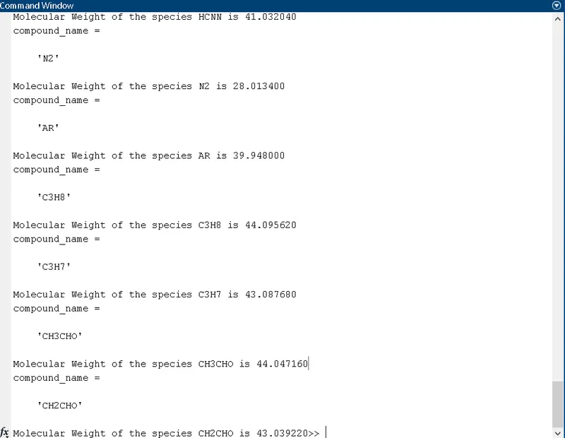
• Develop a code to calculate the molecular weight of each species and display it in the command window.

• To plot the Cp, Enthalpy, and Entropy for the local temperature range (low temperature: high temperature) specific for each species.

• To save the plots as images with appropriate names and dump them in separate folders for each species with a suitable name. All of these should be generated automatically.

File Parsing Theory:

• NASA came up with polynomials that can be used to evaluate thermodynamic properties such as Cp, H, and S. They have also documented the coefficients that are required to evaluate these polynomials for 1000+ species.
• It is the method of splitting the file or other input into a piece of data that can be easily stored or manipulated. By doing this we are going to split a string into parts and then recognize the parts to convert it into something simpler than a string.
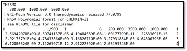
•  Here in this project, we are going to split the NASA thermodynamic data which is having 53 gas species values in 213 lines. To perform the calculation for thermodynamic properties, we need some sort of co-efficient values and temperature ranges which is available in the NASA file. So, we are going to parse the values which are all needed for our calculation from that file.

Specific Heat:

            Specific heat is the amount of heat energy required to raise the temperature of body per unit of mass. Specific heat is also known as specific heat capacity or mass specific heat. In SI units, specific heat is the amount of heat in joules required to raise 1 gram of a substance 1 Kelvin.

Enthalpy:

            When a substance changes at constant pressure, enthalpy tells how much heat and work was added or removed from the substance. Enthalpy is similar to energy but not the same. When a substance grows or shrinks, energy is used up or released.

Entropy:

            The entropy of an object is a measure of the amount of energy that is unavailable to do work. Entropy is also a measure of the number of possible arrangements of atoms a system can have. In this sense, entropy is the measure of uncertainty or randomness.

Gas Constant:

            The gas constant is a physical constant denoted by R and is expressed in terms of units of energy per temperature increment per mole. The gas constant value is equivalent to the Boltzmann constant but expressed as the pressure-volume product instead of energy per increment of temperature per particle.

Molecular Weight:

            Molecular weight is a measure of the sum of the atomic weight values of the atoms in a molecule. Molecular weight is used in chemistry to determine stoichiometry in chemical reactions and equations.

Governing Equations:

Sample NASA data:

Solution Procedure: 

Here some of the Formulae are used to calculate the Enthalpy(H), Entropy(S) and Specific heat(Cp) of a thermodynamic system  

`(Cp)/R = x1 + (x2) T +(x3) T^2 +(x4)T^3+(x5)T^4`

`H/(RT) = x1 + ((x2) T)/2 +((x3) T^2 )/3+((x4)T^3)/4+((x5)T^4)/5+(x6)/T`

`S/R = x1 lnT+ (x2) T +((x3) T^2 )/2+((x4)T^3)/3+((x5)T^4)/4+x7`

where,

Cp = Specific Heat (J/K kg)

H = Enthalpy (J)

S = Entropy (J/K)

R = Universal gas constant = 8.314 (J/mol.K)

T = Temperature (K)

Main Code for Parsing NASA Thermodynamic Data:

clear all
close all
clc

f1 = fopen('THERMO.dat', 'r'); fgetl(f1);
fgetl(f1);
fgetl(f1);
fgetl(f1);
fgetl(f1);


% Extracting all species data

for i = 1:53
    
% Extracting name of gas species

A = fgetl(f1);                  % Reading the sixth line
z = findstr(A,' ');             % Reading the species name
species_name = A(1:z(1)-1);     % Finding out the species name

% Extracting local temperatures of gas species

a = findstr(A,'.');             % Finding string from the line
t1 = A((a(1)-3):a(1)+3);        % Assigning 't' variable for the local temperatures
t1 = str2num(t1);               % Converting string to number
t2 = A(a(3)-4:a(3)+3);
t2 = str2num(t2);
t3 = A(a(2)-4:a(2)+3);
t3 = str2num(t3);

% t1 = Low Temperature
% t2 = Mid Temperature
% t3 = High Temperature

% Extracting co-efficient of gas species

B = fgetl(f1);                  
b = findstr(B,'E');             
a1 = B(1:b(1)+3);               % Assigning 'a' variable for the temperature co-efficients
a1 = str2num(a1);
a2 = B(b(1)+4:b(2)+3);
a2 = str2num(a2);
a3 = B(b(2)+4:b(3)+3);
a3 = str2num(a3);
a4 = B(b(3)+4:b(4)+3);
a4 = str2num(a4);
a5 = B(b(4)+4:b(5)+3);
a5 = str2num(a5);
C = fgetl(f1);
c = findstr(C,'E');
a6 = C(1:c(1)+3);
a6 = str2num(a6);
a7= C(c(1)+4:c(2)+3);
a7 = str2num(a7);
a8 = C(c(2)+4:c(3)+3);
a8 = str2num(a8);
a9 = C(c(3)+4:c(4)+3);
a9 = str2num(a9);
a10 = C(c(4)+4:c(5)+3);
a10 = str2num(a10);
D = fgetl(f1);
d = findstr(D,'E');
a11 = D(1:d(1)+3);
a11 = str2num(a11);
a12 = D(d(1)+4:d(2)+3);
a12 = str2num(a12);
a13 = D(d(2)+4:d(3)+3);
a13 = str2num(a13);
a14 = D(d(3)+4:d(4)+3);
a14 = str2num(a14);

% First 7 are high temperature co-efficients from a1 to a7
% Second 7 are low temperature co-efficients from a8 to a14

% Creating the range of low and high values of local temperatures

T = linspace(t1,t3,1000);

R = 8.314;                  % Universal gas constant in j/mol.k

% Calculation for Specific heat, Enthalpy and Entropy

for i = 1:length(T)
    
    if T(i)>t2
        Cp(i) = (a1 + a2.*T(i) + a3.*T(i).^2 + a4.*T(i).^3 + a5.*T(i).^4)*R;
        H(i) = (a1 + (a2.*T(i))/2 + (a3.*T(i)^2)/3 + (a4.*T(i).^3)/4 + (a5.*T(i).^4)/5 + (a6./T(i)))*R.*T(i); 
        S(i) = a1.*log(T(i)) + a2.*T(i) + (a3.*T(i)^2)/2 + (a4.*T(i)^3)/3 + (a5.*T(i).^4)/4 + a7;
    else
        Cp(i) = (a8 + a9.*T(i) + a10.*T(i).^2 + a11.*T(i).^3 + a12*T(i).^4)*R;
        H(i) = (a8 + (a9.*T(i))/2 + (a10.*T(i).^2)/3 + (a11.*T(i).^3)/4 + (a12.*T(i).^4)/5 + (a13./T(i)))*R.*T(i); 
        S(i) = a8.*log(T(i)) + a9.*T(i) + (a10.*T(i)^2)/2 + (a11.*T(i)^3)/3 + (a12.*T(i).^4)/4 + a14;
    end
end

% Molecular weight calculation

elements = ['H','C','O','N','A','S'];                           % Declaring species elements
atomic_weight = [1.0079 12.0107 15.999 14.0067 39.948 32.065];  % Declaring the atomic weight value
mol_mass = 0;                                                   % Declaring molecular weight to be '0' in initial stage 

for l = 1:length(species_name)
    for m = 1:length(atomic_weight)
        if strcmp(species_name(l), elements(m))
            mol_mass = mol_mass + atomic_weight(m);
            position = m;
        end
    end
    n = str2double(species_name(l));
    if n>1
        mol_mass = mol_mass + atomic_weight(position)*(n-1);
    end
end

% Printing the molecular weight of the gas species in the command window

sprintf('Molecular Weight of %s is %f u',species_name,mol_mass) 

% Creating a folder to save the plots

mkdir(['C:\Program Files\MathWorks MATLAB R2021a v9.10.0.1602886 - CrackzSoft\bin\ou\',species_name])         % Creating a new folder with the species name in the main folder
% cd(sprintf(species_name))   % Changing the directory to the folder of the species name

% Plotting specific heat vs temperature

figure(1)
plot (T,Cp, 'color','b','linewidth',2)
xlabel('Temperature (K)')
ylabel('Specific Heat (J/K Kg)')
title({'Specific Heat vs Temperature',['Species name = ',species_name,' & Molecular weight = ',num2str(mol_mass)]});

% Plotting enthalpy vs temperature

figure(2)
plot (T,H, 'color', 'r','linewidth',2)
xlabel('Temperature (K)')
ylabel('Enthalpy (J/K)')
title({'Enthalpy vs Temperature',['Species name = ',species_name,' & Molecular weight = ',num2str(mol_mass)]});

% Plotting entropy vs temperature

figure(3)
plot (T,S, 'color', 'g','linewidth',2)
xlabel('Temperature (K)')
ylabel('Entropy (J/K)')
title({'Entropy vs Temperature',['Species name = ',species_name,' & Molecular weight = ',num2str(mol_mass)]});

% To change the current directory to the main folder

% oldfolder = cd('I:Chrome DownloadsSkill LyncMATLABFile Parsing Challenge');
cd(['C:\Program Files\MathWorks MATLAB R2021a v9.10.0.1602886 - CrackzSoft\bin\ou\',species_name])         % Creating a new folder with the species name in the main folder
saveas(figure(1),'Cp vs Temp.png')
saveas(figure(2),'Enthalpy vs Temp.png')
saveas(figure(3),'Entropy vs Temp.png')

end

The logic for the code is explained below and file parsing is a beneficial technique. Parsing a file means reading in a data stream of some sort and building an in-memory model of the semantic content of that data. This aims at facilitating performing some kind of transformation on the data and It means, to a computer, about what “reading text” means to a human being. You scan it, from start to finish, and figure out what it means as you go - whether you’re” a person reading text or a computer parsing a file.

Explanation of Code:

1. The program begins with clear all, close all and clc commands to free up the command window and the workspace.
2. We will then read the data from the external NASA thermodynamic data file using fopen command which is used to open the file and fgetl command which is used to read the content in the file line by line.
3. After we use the fopen command we will be assigning to the variable called f1. Thus, the fgetl(f1) is the command acts like a line cursor, which will retrieve the next time while running this command for the second time and so on.
4. Now, we will be skipping the first 5 lines to enter the pattern of values of the respective gas species. We will be using the for loop command to process the same for all the gas species.
5. The name of the gas species we will be found out using findstr command and for finding out the species we are going to locate the string ‘ ’ which is present in after each species name.
6. And then we are going to use A(1:z(1)-1) which tells us the exact location of the species name, using which the name of the gas species is stored in the variable species_name.
7. The local temperatures for the respective gas species is found similarly using findstr command and we are going to locate the string ‘.’ using which we will find out the values of low temperature, mid temperature and high temperature which is assigned to the variables t1, t2 and t3 respectively. But the values we have achieved are string values so we have to change these string values to numeric values using the str2num command.
8. Now, we are going to extract the co-efficient for the gas species in which the co-efficient locations are like in the 2^nd row, next 5 in the 3^rd row and the rest in the 4^th row.
9. We are going to extract these values similarly like we did for finding out the local temperatures by using the findstr and str2num commands and storing it in the variables a1 to a14. For extracting we are going to locate the string ‘E’ which is present in each co-efficient value and so it will be followed for all the coefficients values in the same line and then we can proceed to the next lines.
10. The values from a1 to a7 represent the high-temperature coefficients and the values from a8 to a14 represent the low-temperature coefficients.
11. Temperature range values from low temperature to high temperature is assigned using the linspace command.
12. The for loop command is used to calculate the values of specific heat, enthalpy and entropy and the if-else command is also used to find out the required values if the temperature is below the mid-temperature or above the mid-temperature.
13. In order to calculate the molecular weight of the species we declare the species elements in the form of cell array. Their atomic mass is declared in the form of an array. Then initially molecular weight is declared as zero.
14. Now, for loop command is used to detect if there are more than one species in the variable species_name and the respective values of the gas species values are calculated and found out.
15. After the nested for loop the species_name which is in the form of string is converted as a number with strdouble command. Then the species_name which is now as number is greater than 1, molecular weight is again calculated by having the atomic mass for the current species * n-1
16. The value of the molecular weight is calculated for the respective gas species and is displayed in the command window.
17. Now, we are going to create plots that obtain specific heat, enthalpy and entropy values and save it in the respective species_name folder automatically.
18. In order to create a new folder with the species_name we are going to use the mkdir command so that a new folder is created in the main folder. Now, we have to change the current directory from the main folder to the species_name folder so the cd command is used to do the same.
19. The plots for specific heat vs temperature, enthalpy vs temperature and entropy vs temperature is plotted and the labeling of axis and the naming of the title is also done along with the value of molecular weight.
20. To save the plots in the species_name folder, saveas command is used to save the plots in the current folder. After which to change the current directory to the main folder the oldfolder = cd () command is used.

Output:

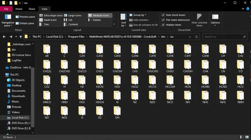
 The Thermodynamic properties of all the polynomials species are saved in a separate folder as shown below

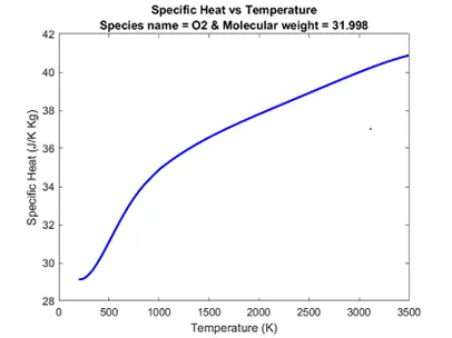
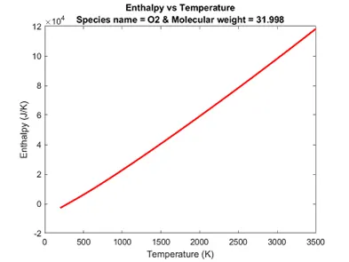
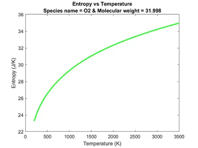
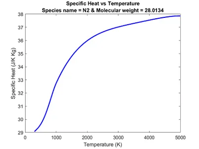
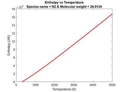
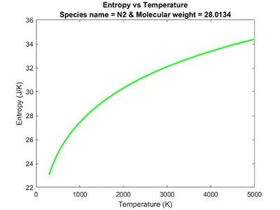
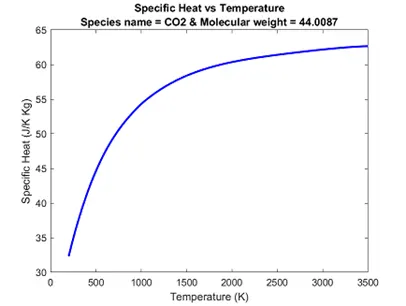
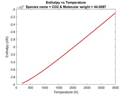
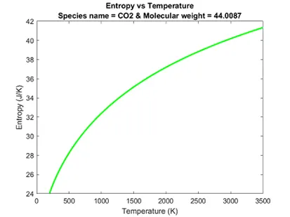
Output for the plots of N2 , O2, and CO2 for the Enthalpy Specific Heat and Entropy:-

Blue color plot - Variation in Enthalpy wrt temperature

Green color plot - Variation in Specific Heat wrt temperature

Red color plot -Variation in Entropy wrt temperature

1)Plot for O2

  

2)Plots for N2

3)Plots for CO2

Output for Molecular weight of the molecule: 

 

Conclusion: