Project
Carry out a system-level simulation of an all-terrain vehicle.
Download the model from the given link:
https://www.mathworks.com/matlabcentral/fileexchange/70576-baja-all-terrain-vehicle-atv-model
Prepare a technical report explaining the model properties & comments on the results.
Ans:
Aim of the Project:- To prepare a technical report of an all-terrain vehicle under the different conditions.
Description:
Inside the CVT(Continuously variable transmission) model:
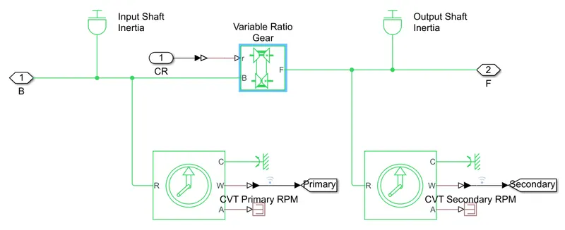
Fig.1 Inside the CVT model
Variable Ratio Gear:
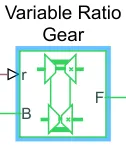
Represents a variable ratio gearbox such as implemented by mechanical belt CVT, electric, or hydraulic transmissions. The physical signal input r defines the ratio of input to output angular shaft velocities.
Connections B (base) and F (follower) are mechanical rotational conserving ports. Specify the relation between base and follower rotation directions with the Output shaft rotates parameter.
Ideal Rotational Motion Sensor:
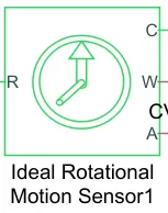
This block measures angular velocity or angle in a mechanical rotational network. The sensor is ideal since it does not account for inertia, friction, delays, energy consumption, and so on.
The physical signal ports W and A report the angular velocity and angular displacement, respectively, of port R relative to port C. The measurement is positive when the motion at R is greater than the motion at C.
Inside the Vehicle body model:
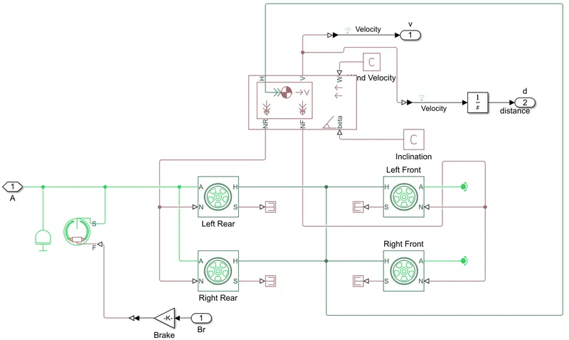
Fig.2 Inside the Vehicle body
Vehicle Body:
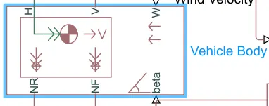
Represents a two-axle vehicle body in longitudinal motion. The block accounts for body mass, aerodynamic drag, road incline, and weight distribution between axles due to acceleration and road profile. The vehicle can have the same or a different number of wheels on each axle. Optionally include pitch and suspension dynamics or additional variable mass and inertia. The vehicle does not move vertically relative to the ground.
Connection H is the mechanical translational conserving port associated with the horizontal motion of the vehicle body. The resulting traction motion developed by tires should be connected to this port. Connections V, NF, and NR are physical signal output ports for vehicle velocity and front and rear normal wheel forces, respectively. Wheel forces are considered positive if acting downwards. Connections W and beta are physical signal input ports corresponding to headwind speed and road inclination angle, respectively. If variable mass is modeled, the physical signal input ports CG and M are exposed. CG accepts a two- element vector representing the x and y distance offsets from vehicle CG to additional load mass CG. M represents the additional mass. If both variable mass and pitch dynamics are included, the physical signal port J accepts the inertia of the additional mass about its own CG.
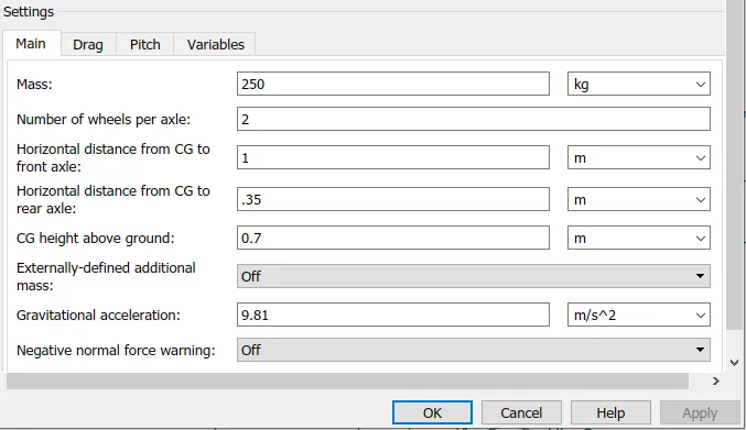
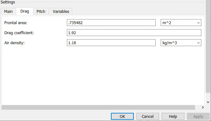
Fig.3 Input of vehicle body parameters
Tire:
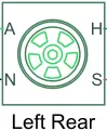
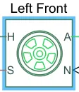
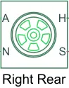
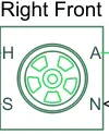
Represents the longitudinal behavior of a highway tire characterized by the tire Magic Formula. The block is built from Tire-Road Interaction (Magic Formula) and Simscape Foundation Library Wheel and Axle blocks. Optionally, the effects of tire inertia, stiffness, and damping can be included.
Connection A is the mechanical rotational conserving port for the wheel axle. Connection H is the mechanical translational conserving port for the wheel hub through which the thrust developed by the tire is applied to the vehicle. Connection N is a physical signal input port that applies the normal force acting on the tire. The force is considered positive if it acts downwards. Connection S is a physical signal output port that reports the tire slip. Optionally expose physical signal port M by setting Parameterize by to Physical signal Magic Formula coefficients. Physical signal port M accepts a four element vector corresponding to the B, C, D, and E Magic Formula coefficients.
Double Shoe Brake:
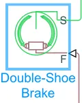
Represents a brake arranged as two pivoted rigid shoes symmetrically installed inside or outside a drum and operated by one actuator. The actuator force causes the shoes to exert a friction torque on a shaft connected to the drum.
Connection S is a conserving rotational terminal associated with the drum shaft. Connection F is a physical signal port representing the force input to the actuator. Positive force creates friction torque that resists shaft rotation. Optionally include thermal effects and expose thermal conserving port H by setting Thermal port to Model.
CASE 1: Simulink model for BAJA ATV with CVT using Dashboard
taking Brake input= 0, and Throttle input= 0.5
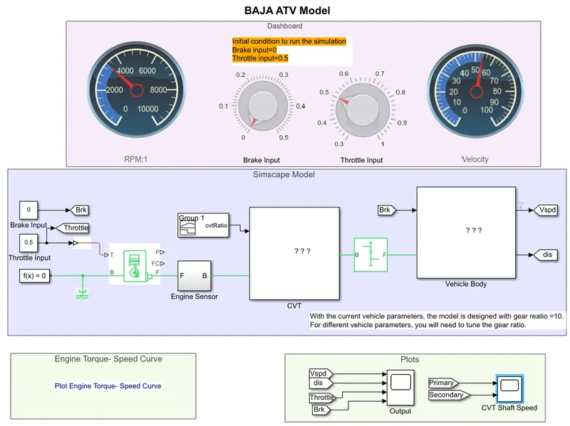
Fig.4 BAJA ATV model for CASE 1
In this model the dashboard is provided to control the inputs i,e here brake and throttle are the two inputs which we used. This dashboard helps us to verify the outputs in real time situation. And we gave brake input as 0 and throttle input as 0.5 as by the default values. Also we use signal builder block replacing a saperate constant block, a variator is provided to change the input values in real time situation.
Input of Torque vs Engine speed:
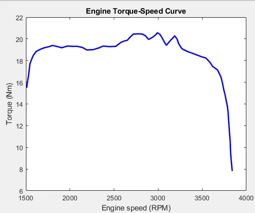
It shows a input values of Engine torque and speed curve in the form of graph. If we need perticular values from this image we must use grabit option.
Brake and Throttle input:
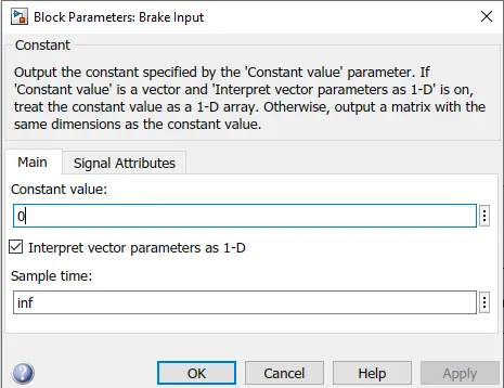
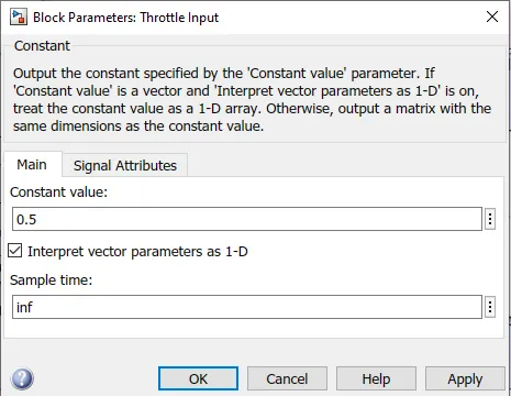
Here we gave 0 value to the brake input and 0.5 value for throttle input.
Output of Vehicle speed for CASE 1:
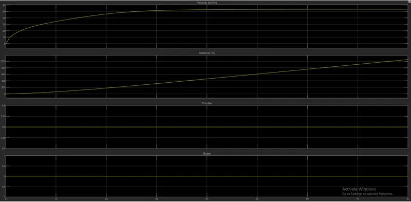
Fig.5 Output of CASE 1
Result:
From the above graph we can observe that the vehicle speed is increased from 0 to 52kmph fot constant 0.5 throttle value and 0 brake input. If we increase the brake from 0 onwards the vehicle speed goes decreases accordingly, and also if we reduce the throttle value then also the speed of the vehicle starts decreasing. This graph explains relation of vehicle speed with respect to throttle and brake input.
-------------------------------------------------------------------------------------------------------------------------------------------
CASE 2: Simulink model for BAJA ATV with CVT using Dashboard
taking Brake input= 0, and Throttle input= 0.3
Simulink model:
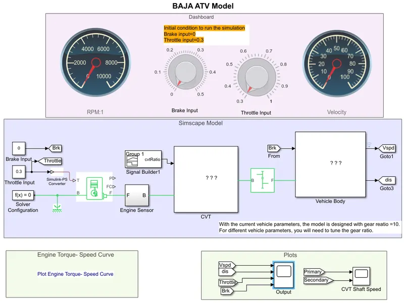
Fig.6 BAJA ATV model for CASE 2
In this model the dashboard is provided to control the inputs i,e here brake and throttle are the two inputs which we used. This dashboard helps us to verify the outputs in real time situation. And we gave brake input as 0 and throttle input as 0.3 as per the condition. Also we use signal builder block replacing a saperate constant block, a variator is provided to change the input values in real time situation.
Output:
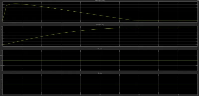
Fig.7 Output of CASE 2
Result:
From the above graph we can observe that the vehicle speed is increased from 0 to 5.2 kmph fot constant 0.3 throttle value and 0 brake input. If we increase the brake from 0 onwards the vehicle speed goes decreases accordingly, and also if we reduce the throttle value then also the speed of the vehicle starts decreasing. This graph explains relation of vehicle speed with respect to throttle and brake input.
-------------------------------------------------------------------------------------------------------------------------------------------------
CASE 3: Simulink model for BAJA ATV with CVT using Dashboard
taking Brake input= 0.2, and Throttle input= 0.3
Simulink model:
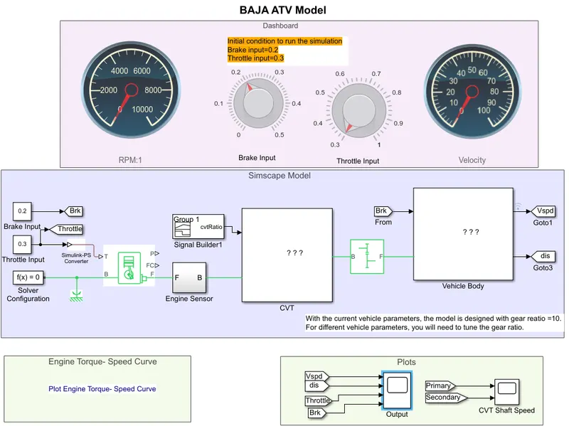
Fig.8 BAJA ATV model for CASE 3
In this model the dashboard is provided to control the inputs i,e here brake and throttle are the two inputs which we used. This dashboard helps us to verify the outputs in real time situation. And we gave brake input as 0.2 and throttle input as 0.3 as per the condition. Also we use signal builder block replacing a saperate constant block, a variator is provided to change the input values in real time situation.
Output:
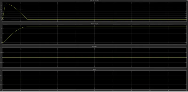
Fig.9 Output of CASE 3
Result:
From the above graph we can observe that the vehicle speed is increased from 0 to 5.2 kmph fot constant 0.3 throttle value and 0.2 brake input. If we increase the brake from 0 onwards the vehicle speed goes decreases accordingly, and also if we reduce the throttle value then also the speed of the vehicle starts decreasing. This graph explains relation of vehicle speed with respect to throttle and brake input.
Conclusion:
Hence we successfully analysed in three different conditions and observed the speed of the vehicle as per the conditions. For case1 we gave brake and throttle of 0 & 0.5 respectively, and got output of vehicle speed as 52 kmph constant. For case2 we did brake and throttle input of 0 & 0.3 respectively, and output of 5.2 kmph between 0-3 seconds. For case3 we gave brake and throttle input of 0.2 & 0.3 respectively, and got output in the form of vehicle speed i.e 3.7 kmph between 0-3 seconds.